
Monitoring of Grinding Burn by AE and Vibration Signals
Rodolpho F. Godoy Neto
1
, Marcelo Marchi
1
, Cesar Martins
2
, Paulo R. Aguiar
2
and Eduardo Bianchi
1
1
Mechanical Department, School of Engineering, Univ. Estadual Paulista - UNESP,
Av. Luiz E.C. Coube, 14-01, 17033-0360, Bauru – SP, Brazil
2
Electrical Engineering Department, School of Engineering, Univ. Estadual Paulista - UNESP,
Av. Luiz E.C. Coube, 14-01, 17033-0360, Bauru – SP, Brazil
Keywords: Neural Network Application, Monitoring, Acoustic Emission, Grinding Process, Burn.
Abstract: The grinding process is widely used in surface finishing of steel parts and corresponds to one of the last
steps in the manufacturing process. Thus, it’s essential to have a reliable monitoring of this process. In
grinding of metals, the phenomenon of burn is one of the worst faults to be avoided. Therefore, a monitoring
system able to identify this phenomenon would be of great importance for the process. Thus, the aim of this
work is the monitoring of burn during the grinding process through an intelligent system that uses acoustic
emission (AE) and vibration signals as inputs. Tests were performed on a surface grinding machine,
workpiece SAE 1020 and aluminum oxide grinding wheel were used. The acquisition of the vibration
signals and AE was done by means of an oscilloscope with a sampling rate of 2MHz. By analyzing the
frequency spectra of these signals it was possible to determine the frequency bands that best characterized
the phenomenon of burn. These bands were used as inputs to an artificial neural networks capable of
classifying the surface condition of the part. The results of this study allowed characterizing the surface of
the work piece into three groups: No burn, burn and high surface roughness. The selected neural model has
produced good results for classifying the three patterns studied.
1 INTRODUCTION
Grinding is one of the most finishing processes used
in the manufacture of precision mechanical
components. It is the last stage in the manufacturing
chain, which is why it affords a high added value to
the end product. Despite its importance and
popularity, grinding still remains as one of the most
difficult and least understood processes in addition
to the function of solving the problems of time and
quality of the entire production sequence (Irani et al.
2005; Aguiar et al. 2010).
According to (Liao et al. 2008), grinding is one
of the most complicated process, mostly due to the
fact that a grinding operation is performed by a
grinding wheel which is composed of many tiny,
irregular shaped, and randomly positioned and
oriented abrasives (also called grits) bonded by some
medium. Thus, there are many variables that make it
difficult to choose the optimal parameters in a
simple way.
Since a reduction of the production costs and an
increase in the quality of the machined parts are
expected, the automated detection of the machining
process malfunctions has become of great interest
among scientists and industrialists. By the use of a
large variety of sensors, monitoring of machining
processes represents the prime step for reduction of
poor quality and hence a reduction of costs (Axinte
et al. 2004).
One of the most critical problems in the
intelligent grinding process implementation is the
automatic detection of surface burn in the parts. The
burn occurs during the cutting of the part by the
grinding wheel when the amount of energy
generated in the contact area produces an increase of
temperature enough to produce a change of phase in
the material. Such occurrence can visually be
observed by the bluish temper color on the part
surface (Aguiar et al. 2002). Grinding burn also has
an adverse effect on component in-service strength
and fatigue properties. When grinding becomes
abusive the grinding temperature can easily rise to
more than 800 C. Due to the effects of elevated
temperature, the surface of the workpiece may burn
and the deterioration of the surface becomes evident.
Workpiece burn during the grinding process is
272
F. Godoy Neto R., Marchi M., Martins C., R. Aguiar P. and Bianchi E..
Monitoring of Grinding Burn by AE and Vibration Signals.
DOI: 10.5220/0004753602720279
In Proceedings of the 6th International Conference on Agents and Artificial Intelligence (ICAART-2014), pages 272-279
ISBN: 978-989-758-015-4
Copyright
c
2014 SCITEPRESS (Science and Technology Publications, Lda.)

essentially an irreversible change in the
microstructure of a surface layer (Liu et al. 2005).
Therefore, the grinding burn control and monitoring
is of great interest to all industries dependent on the
grinding process, thus leading to a reduction in scrap
rate and production costs.
The main difficulty of controlling damages
caused in the grinding process is the lack of a
reliable method in supplying feedback in real time
during the process. Since the grinding process
causes intensive mechanical vibration and strong
acoustic emission, these signals can be picked up
easily and recorded by commercially available
instruments.
According to (Babel et al. 2013), in light of its
superior sensitivity to the multitude of fine dynamic
interactions between the wheel and the workpiece,
acoustic emission (AE) has emerged as a valuable
tool in a host of monitoring applications in grinding.
Typical examples include in-process wheel
mapping, and the sensing of wheel–work contact,
wheel loading, chatter and thermal damage. Still, the
authors report that in many applications, it suffices
to examine the signal in terms of time-averaged
indices, while others necessitate frequency domain
analyses of the raw AE signal, as the relevant
information is embedded in the spectral components
of the signal. In either case, due to the complex
nature of grinding processes, the challenge in the
effective and reliable application of AE lies in the
identification and interpretation of signatures
pertinent to the process responses that are of interest.
On the other hand, vibration is produced by
cyclic variations in the dynamic components of the
cutting forces, resulting from periodic wave
motions. The nature of vibration signals arising from
the metal cutting process incorporates free, forced,
periodic, and random types of vibration. Direct
measurement of vibration is difficult to achieve
because the vibration mode is frequency dependent.
Hence, related parameters are measured such as the
rate at which dynamic forces change per unit time
(acceleration) and the characteristics of the vibration
are derived from the patterns obtained (Dimla, Snr.
2002).
Several investigations have been carried out to
correlate vibration signals to the characteristics of
maching processes. For exemple, Yamamoto et al.
apud (Hassui & Diniz 2003) monitored the wheel
vibration (they fixed the sensor on the wheel
bearing) to detect the clogging of the wheel pores by
chips. Aiming towards this goal, they used adaptive
digital filters and created an index, based on the
outputs of these filters, called index of the signal
pattern. This index showed to have a good
relationship with the volume of chips clogged in the
wheel. (Hassui et al. 1998) proved that the RMS
signal of the workpiece vibration (they fixed the
sensor on the workpiece tailstock) presents better
relationship with wheel wear than acoustic emission.
Besides, the sensitivity of the vibration signal to
detect the wheel–workpiece moment of contact and
the moment of spark out end is as good as acoustic
emission sensitivity. (Hassui & Diniz 2003) tested
the ability of the vibration signal to follow the
changes of workpiece surface roughness and
circularity, in order to verify the possibility of using
it for the automatic definition of the dressing
moment.The results showed good correlation of
vibration signals with surface roughness and wheel
condition.
According to (Teti et al. 2010), it is generally
acknowledged that reliable process condition
monitoring based on a single signal feature (SF) is
not feasible. Therefore, the calculation of a sufficient
number of SFs related to the tool and/or process
conditions is a key issue in machining monitoring
systems. This is obtained through signal processing
methods that comprise pre-processing (filtering,
amplification, A/D conversion, and segmentation)
including, on occasion, signal transformation into
frequency or time–frequency domain (Fourier
transform, wavelet transform, etc).
One of the most used signal feature in maching
monitoring systems is the root mean square (RMS)
value, and it can be expressed as shown in equation
1.
1
∆
∆
(1)
where t is the integration time constant, and f
raw
is
the raw signal (Kim et al. 2001).
Thus, acoustic emission and vibration signals
have their own and interesting characteristics, which
adequately extracted and related to the studied
phenomena can provide valuable information to the
grinding process monitoring. This work aims at
monitoring workpiece burn during the grinding
process through neural modelling that uses features
of the acoustic emission (AE) and vibration signals
as inputs.
What makes this work distinguishible from
others is the use of vibration signal along with AE
signal. The former has not yet been employed in
grinding burn detection. Besides, study on frequency
domain for both signal that closely relates frequency
bands to bun, non burn and high surface roughness
MonitoringofGrindingBurnbyAEandVibrationSignals
273

values has not been carried out either. The selection
of frequency bands from the signal espectrum aims
to better extract the signal features for the classes
studied. Another contribuition of this work is related
to the types of classes, i.e., the models are able to
classify parts with high surface roughness values (no
visible burn), visible burn occurrence and normal
operation. It is worth mentioning that thermal
sensing, such as thermocouples inserted in the
workpiece or tool could produce good results as well
in monitoring the grinding burn. However, such
techniques are genererally invasive and, therefore,
infeaseble in most practical implementation.
2 NEURAL NETWORKS
IN MACHINING PROCESSES
According to (Teti et al. 2010), in monitoring and
control activities for modern untended
manufacturing systems, the role of cognitive
computing methods employed in the implementation
of intelligent sensors and sensorial systems is
fundamental. A conspicuous number of schemes,
techniques and paradigms have been used to develop
decision-making support systems functional to come
to a conclusion on machining process conditions
based on sensor signals data features. The cognitive
paradigms most frequently employed for the purpose
of sensor monitoring in machining, including neural
networks, fuzzy logic, genetic algorithms and hybrid
systems able to combine the capabilities of the
various cognitive methods.
Artificial neural networks (ANNs) are adaptive
and have parallel information-processing structures
with the ability to build functional relationships
between data and to provide powerful tools for
nonlinear, multidimensional interpolations. This
aspect of neural networks makes it possible to
capture and interpret the existing highly complex
nonlinear relationships between input and output
parameters that are frequently poorly understood. An
ANN is a system consisting of processing elements
(PE) with links between them. A certain
arrangement of the PEs and links produce a certain
ANN model, suitable for certain tasks (Ahmadzadeh
& Lundberg 2013).
Anns have been accepted as a very good tool that
can be applied to many nonlinear problems, where
finding solutions using traditional techniques are
cumbersome or impossible. Examples of applied
areas of nns include robotics, control, and system
identification. They have been successfully used in
condition monitoring and fault diagnosis in
machining processes. These applications have
usually used the pattern recognition approach
combined with the classification ability of anns
(marzi 2008).
Similar work on classification of grinding burn
can be found in (Spadotto et al. 2008), where the
authors perform only the classification of burn
degrees (slight burn, medium burn, severe burn and
non burn) of the part ground by using acoustic
emission and power signals statistics as inputs to the
neural network models. The results were good,
reaching a success rate of 93.5 % for model II,
which employs a statistic named DPO proposed by
(Aguiar et al. 2002), composed of the multiplication
between standard deviation of RMS AE and
maximum value of grinding power in the grinding
pass. Another similar work is presented by (Dotto et
al. 2003) in which a neural network model having
the RMS AE and grinding power as inputs is used to
classify burn and non burn condition of the parts
ground. Good response of the model can be
observed in the regions charts, where burning and
non burning occurrence were classified. The
investigation in (Kwak & Ha 2004) proposed a
diagnostic scheme of a grinding states (chatter,
vibration and grinding burn) by the neural network
using power and AE signals. The maximum
successful diagnosis was about 95 %. Other
investigations related to the topic of this work can
also be found. However, none of them has used the
vibration signal as well as verified the condition of
high surface roughness values of the work piece
ground.
3 MATERIALS AND METHODS
3.1 Experiments
The experimental tests were carried out in a surface
grinding machine. Each test consisted of a single
grinding pass across the workpiece length. Preceding
each test, a single-point diamond dresser performed
the dressing of the grinding wheel. Table 1 shows
the grinding condition of each test.
An acoustic emission sensor and a processing
signal unit, from Sensis manufacturer, model DM-
42, were employed in the tests. Also, a vibration
sensor, model 353B03 and a conditioning signal
unit, from PCB Piezotronic, were used. An
oscilloscope, model DL850, from Yokogawa,
collected both raw signals, at a sampling rate of 2
MHz. The sensors were fixed on the workpiece
holder and tested for good signal sensitivity and
ICAART2014-InternationalConferenceonAgentsandArtificialIntelligence
274
without saturation.
Workpieces of SAE 1020 steel were ground with
an aluminum oxide grinding wheel, model 38A150-
LVH, from Norton, and cutting fluid was employed
(Emulsion water-oil of 4 %). The following grinding
parameters were used in the 13 tests: peripheral
speed of the grinding wheel – 30.78 m/s; workpiece
speed – 0.04 m/s; grinding wheel diameter – 326.64
mm; wheel width – 24.09 mm; workpiece
dimensions – 152.64 mm length and 13.01 mm
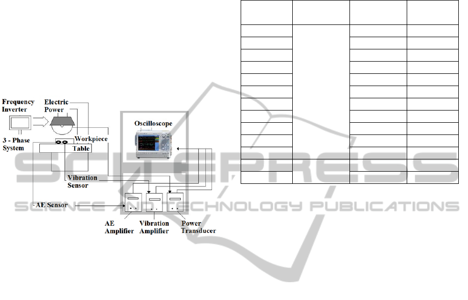
width. The schematic diagram in Figure 1 shows the
experimental test setup used in this work.
Figure 1: Experimental setup.
Following the experiments, the average surface
roughness (Ra) for each workiece was measured,
using a Taylor Hobson Surtronic 3+ precision
instrument. A sampling length of 1.6 mm and cut-off
of 0.8 mm were used, following the
recommendations of the ISO 4288-1996 standard.
Each workpiece surface length was equally divided
into 30 parts, where 3 surface roughness
measurements were taken from each part. Thus, the
mean value and standard deviation of each part were
calculated, allowing the assessment of the ground
workpiece regarding this important parameter. In
addition to the surface roughness measurements, the
visual inspection of each workpiece surface was
carefully carried out as well as all workpiece
surfaces were digitally photographed for further
analysis.
Table 1 shows information of the 13 tests, where
the cutting geometry means whether the grinding
wheel cut the workpiece in the conventional way,
i.e., flat geometry, or the workpiece was precisely
inclined to allow a ramp-cutting geometry. The latter
way, there are two cutting depths regarding the onset
and the end of the cutting, respectively. In Table 1,
HR stands for high surface roughness value, which
was so considered workpieces with this value higher
than 1.6 m and with no visible burn. Workpieces
with visible burn was considered as burn, and those
with no visible burn at all were classified as no burn.
Table 1: Information of the tests.
Test Cutting
Geometry
Depth of
Cut (m)
Surface
condition
1
Flat
10 No burn
2 20 No burn
3 30 Burn
4 40 Burn
5 40 No burn
6 30 No burn
7 20 No burn
8 10 No burn
9 20 No burn
10 30 No burn
11 55 HR
12 Ramp
20-70 HR
13 30-80 HR
3.2 Selection of Frequency Bands
and RMS Vectors
The data acquisition produced vector of 20 million
of samples for each machined workpiece. Subsets of
400,000 samples were selected from each test vector
and for each surface condition (No burn, burn and
high surface roughness) for further digital
processing. The data sets from the tests were
digitally processed in MATLAB. A study on the
signals spectra was performed in order to identify
frequency bands more strongly related to the burn
phenomenon in surface grinding. The Fast Fourier
Transform (FFT) algorithm was implemented in
MATLAB routine for each surface condition. The
RMS values of each signal (AE and vibration) were
used as reference to pick the right position from
which the 8192-block FFT, Hanning window, was
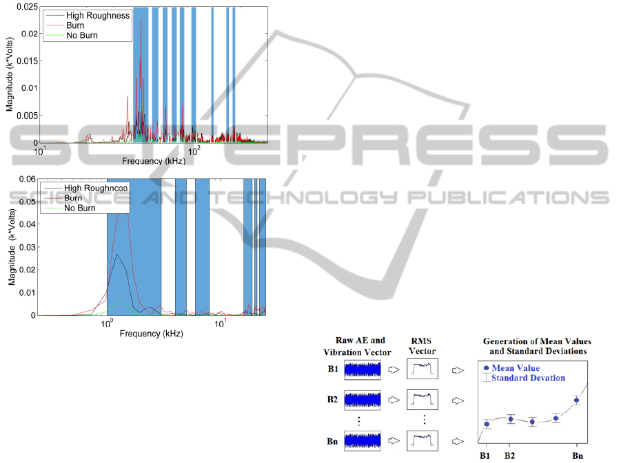
performed. The spectra for AE and vibration signals
are shown in Figure 2, where AE is within a
frequency range of 20 kHz to 300 kHz and vibration
of 1 kHz to 25 kHz, given by the sensors and
process characteristics. Frequency bands were then
selected from the spectrum of each signal, where
nine frequency bands were chosen for the AE signal
and six for the vibration signal, as shown in Figure 2
by the shade areas. The justification for frequency
band selection is based on obtaining the best feature
extraction that represents the classes studied (no
burn, burn, high surface roughness). The criterion
used in the frequency band selection was looking for
the frequency windows on which the magnitudes of
the signal for each class presented good differences.
MonitoringofGrindingBurnbyAEandVibrationSignals
275
Also, a minimum of overlapping among the three
classes spectra was sought. These frequency bands,
in kHz, are as following for AE: 40-51, 53-59, 62-
68, 71-78, 80-87, 95-104, 128-135, 160-170, and
176-186. The frequency bands selected, in kHz, for
vibration are: 1-3, 4-5, 6-8, 16-19, 20-21, and 22-25.
It is worth mentioning that there are other frequency
bands, which could be studied as well, but they will
be considered for further study.
Figure 2: Frequency spectra of three conditions and the
chosen frequency bands. (a) AE; (b) Vibration.
Three vectors of 400,000 samples each were
extracted from the raw signals (AE and vibration)
for each workpiece surface condition (no burn, burn,
and high roughness). This procedure was based on
three regions along a given ground workpiece,
which represented a certain surface condition.
Butterworth digital filters, order 6, for each
frequency band previously selected, were applied to
those vectors, and therefore new filtered vectors
were generated. The RMS values were obtained
using a block length of 2048 from the filtered
vectors for each workpiece surface condition.
Therefore, three RMS vectors were generated for
each surface condition from which the mean value
and standard deviation were calculated. Figure 3
depicts the procedure herein described. In this
figure, B1 to Bn stand for the frequency bands
selected for study.
3.3 Neural Network Models
Three types of MLP neural models were considered
for comparison in order to choose the best
classification model. Before building the NN
models, the analysis of the RMS values in function
of the frequency bands was carried out, and two
frequency bands for each signal (AE and vibration)
were selected for the models. Thus, the first NN
model consisted of 1 input (RMS values) and 3
outputs (No burn, burn, and high roughness), and it
was obtained by testing into the model each RMS
vector filtered out for the 4 frequency bands selected
previously. The second NN model was composed of
2 inputs (2 RMS values) and 3 outputs (as in the first
model), and it was obtained by testing two RMS
vectors into the model, as inputs, filtered out for the
4 frequency bands aforementioned. Finally, the third
model comprised of four RMS vectors at each
frequency band selected, as inputs, and 3 outputs (as
in the first and second models). An algorithm for
training and testing the models in MATLAB was
developed, where the number of neurons (5, 10, 15,
20 and 25) and hidden layers (1 to 3) were varied.
The Levenberg-Marquardt algorithm for training the
neural models was used. In addition, sigmoid
tangent activation function for the neurons of the
hidden layers and linear activation function for the
neurons of the output layer were found more
suitable.
Figure 4: RMS values as a function of frequency bands;
(a) AE; (b) vibration.
The input RMS vectors for training, testing and
validating the neural models were obtained by
dividing every RMS vector at each frequency band
selected into 200 equally parts. This was done for
both signals acquired (AE and vibration) in the 13
experimental tests. Therefore, a number of 2,600
samples for each RMS vector and for each
frequency band was obtained, resulting in the total
of 10,400 RMS values (4 frequency bands selected
and further described). Of course, depending on the
model considered, a different number of samples
will be used in the training process, as described
(a)
(b)
ICAART2014-InternationalConferenceonAgentsandArtificialIntelligence
276
previously. The total data obtained from the
aforementioned procedure was then divided
randomly, with 60 % used for NN model training
and 20 % for validation. The remaining 20 % was
used to test the ANN to confirm its satisfactory
performance as well as to build the confusion
matrices of the models.
To train the MLP networks, ranges representing
the values 0 and 1 were defined. Thus, values
between -0.50 and 0.50 represent the output 0, while
values within the interval of 0.51 and 1.50 represent
the output 1.
4 RESULTS AND DISCUSSION
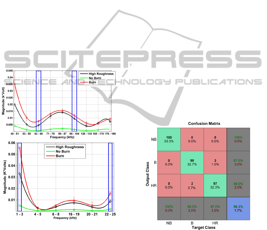
Figure 4(a) and 4(b) depicts the curves of the RMS
values for the nine and six frequency bands selected
for AE and vibration, respectively.
Figure 4: RMS values as a function of frequency bands;
(a) AE; (b) vibration.
The choice of the best frequency bands was based on
the observation of the signal magnitudes and
standard deviations at each frequency band. In other
words, a good situation was considered when the
signal magnitude increased according to the
following order of surface condition: no burn, high
roughness and burn. Also, the proximity of the
curves as well as the standard deviation were taken
into account, i.e., a small standard deviation and
non-overlapping of the curves were sought. Thus,
the frequency bands selected for the models were the
following: 62-68 kHz (B2 – AE), 95 kHz – 104 kHz
(B6 – AE), 1 kHz – 3 kHz (B1 – VIB), and 22 kHz –
25 kHz (B6 – VIB). These frequency bands are
indicated in Figure 4 as blue rectangles.
The results of the best neural models are
presented in Table 2, where it can be observed that
the combination of the AE and vibration signals in
the frequency bands selected (shown in Figure 4),
produced the best classification result (98.3 %) in
model A. Notwithstanding, the result of model 2
also shows a high level of classification (96.0 %).
Besides, model B has only 2 inputs, i.e., AE at 62
kHz - 68 kHz and vibration at 1 kHz – 3 kHz, which
is more suitable for hardware implementation.
Based on the results of models A and B, one can
argue that frequency band of 62 kHz – 68 kHz for
AE and 1 kHz – 3 kHz for vibration are good in the
feature extraction for this work.
Model C, however, presented a low success rate
of classification. That is due to the frequency bands
used in this model are not much representative of the
workpiece conditions.
Figure 5 shows the confusion matrix for model
A, which was obtained from 20 % of data set not
presented to the network-training phase.
Figure 5: Confusion Matrix for Model A (B=burn, NB=No
burn, HR=High roughness value).
It can be observed in the figure the good capacity of
pattern classification of the network, especially in
the class of no burn (NB) in which the success rate
of 100 % was achieved. The network, however, has
produced two false negatives for the burn class (B),
which were classified as high roughness (HR). Also,
three false negatives are observed for the high
(a)
(b)
MonitoringofGrindingBurnbyAEandVibrationSignals
277
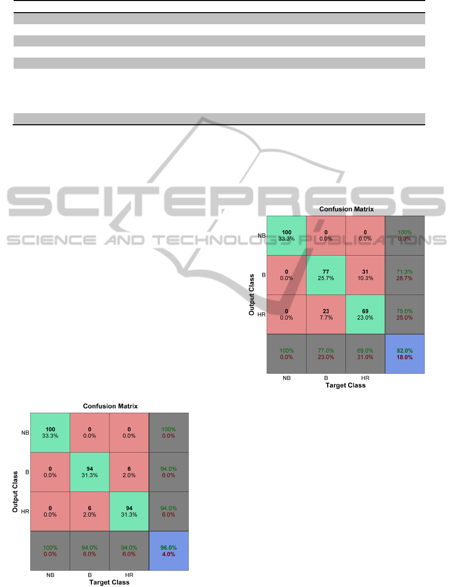
Table 2: Results of the best neural models.
Name Model A Model B Model C
Input Parameter Mean RMS value of AE and Vibration signals
Structure 10
–
10
–
5 25
–
0
–
0 3
–
3
–
0
Train. Function Levenber
g
-
M
arquardt Backpropa
g
ation
Max epochs 1000
Inputs 4 2 2
Frequency Bands
AE: 62kHz
–
68 kHz
95kHz – 104 kHz
VIB: 1kHz – 3kHz;
22kHz
–
25kHz
AE: 62kHz
–
68 kHz
VIB: 1kHz – 3kHz
AE: 95kHz
–
104 kHz
VIB: 22kHz – 25kHz
Overall Result 98.3 % 96.0 % 82.0 %
roughness class, which were classified as burn class.
Both kinds of errors could not be of concern in the
industrial environmental, since it would not
compromise the quality of the part being
manufactured.
The confusion matrix for model B is shown in
Figure 6. In this model, a greater number of false
negatives is observed for the same classes of model
A. On the other hand, this model has only two
inputs, which makes it more attractive for hardware
implementation.
The confusion matrix for model C is presented in
Figure 7, where one can clearly see the high number
of false negatives for both classes of burn and high
roughness. However, the success rate of 100 % for
no burn class was similarly achieved.
The models with one input have shown high
level of errors, and thus they were not presented.
Comparing the results of this work with the
investigations of (Kwak & Ha 2004) and (Spadotto
et al. 2008), it can be observed an improvement
in classifying the burn occurrence, i.e., model A
Figure 6: Confusion Matrix for Model B (B=burn, NB=No
burn, HR=High roughness value).
presented a success rate of 98.3 % against 95 % and
93.5 %, respectively. In addition, this investigation
adds an important class of high surface roughness to
the neural models, which becomes the monitoring
system even more effective.
Figure 7: Confusion Matrix for Model C (B=burn, NB=No
burn, HR=High roughness value).
5 CONCLUSIONS
The frequency content of the AE and vibration
signals showed different behavior for the three
surface conditions studied. Based on this analysis,
frequency bands could be selected for the neural
models, i.e., 62-68 kHz (B2 – AE), 95 kHz – 104
kHz (B6 – AE), 1 kHz – 3 kHz (B1 – VIB), and 22
kHz – 25 kHz (B6 – VIB).
The results showed that neural model A
presented a success rate of 98.3 %, which had the
four RMS inputs (2 AE and 2 VIB). However, a
small number of false negatives were observed in
the burn class as well as in the high roughness class,
which would not necessarily compromise the quality
ICAART2014-InternationalConferenceonAgentsandArtificialIntelligence
278

of the part being manufactured. Also, model B
produced good results with a success rate of 96.0 %,
but an increased number of false negatives. This
model had only two inputs (1 AE and 1 VIB).
Nonetheless, the hardware implementation of model
B would be more interesting. Model C, however,
presented low success rate of classification and must
be discarded.
From model A and B, one can be argued that
frequency band of 62 kHz – 68 kHz for AE and 1
kHz – 3 kHz for vibration are good in the feature
extraction for this work.
As discussed in the previous section, the results
of this work have proved superior when compared
with the investigations of (Kwak & Ha 2004) and
(Spadotto et al. 2008). The extraction of the best
signals features from the spectra as well as the use of
vibration signal along with AE produced better
classification results.
Based on one of the best models obtained, it
would be possible to implement it into a hardware
that could provide information in real-time to
operator in order to make adjustments and possibly
avoid burning. In the case of burn classification has
been made, the part should be discarded.
ACKNOWLEDGEMENTS
The authors are indebted to FAPESP, CNPq and
CAPES, Brazilian agencies that have supported this
work. Also, thanks go to the NORTON Company,
from Saint Gobain Group, for donating the wheel.
REFERENCES
Aguiar, P.R., Bianchi, E.C. & Oliveira, J.F.G., 2002. A
method for burning detection in grinding process using
acoustic emission and effective electric power signals.
Manufacturing Systems, 31(3), pp.253–257.
Aguiar, P.R. De, Paula, W.C.F. De & Bianchi, E.C., 2010.
Analysis of Forecasting Capabilities of Ground
Surfaces Valuation Using Artificial Neural Networks.
J. of the Braz. Soc. of Mech. Sci. & Eng., XXXII(2),
pp.146–153.
Ahmadzadeh, F. & Lundberg, J., 2013. Remaining useful
life prediction of grinding mill liners using an artificial
neural network. Minerals Engineering, 53, pp.1–8.
Axinte, D. a et al., 2004. Process monitoring to assist the
workpiece surface quality in machining. International
Journal of Machine Tools and Manufacture, 44(10),
pp.1091–1108.
Babel, R., Koshy, P. & Weiss, M., 2013. Acoustic
emission spikes at workpiece edges in grinding: Origin
and applications. International Journal of Machine
Tools and Manufacture, 64, pp.96–101.
Dimla, Snr., D.E., 2002. The Correlation of Vibration
Signal Features to Cutting Tool Wear in a Metal
Turning Operation. The International Journal of
Advanced Manufacturing Technology, 19(10), pp.705–
713.
Dotto, F. et al., 2003. Automatic detection of thermal
damage in grinding process by artificial neural
network. Revista Escola de Minas, 56(4), pp.295–300.
Hassui, a. et al., 1998. Experimental evaluation on
grinding wheel wear through vibration and acoustic
emission. Wear, 217(1), pp.7–14.
Hassui, a. & Diniz, a. E., 2003. Correlating surface
roughness and vibration on plunge cylindrical grinding
of steel. International Journal of Machine Tools and
Manufacture, 43(8), pp.855–862.
Irani, R. a., Bauer, R.J. & Warkentin, a., 2005. A review
of cutting fluid application in the grinding process.
International Journal of Machine Tools and
Manufacture, 45(15), pp.1696–1705.
Kim, H.. et al., 2001. Process monitoring of centerless
grinding using acoustic emission. Journal of Materials
Processing Technology, 111(1-3), pp.273–278.
Kwak, J.-S. & Ha, M.-K., 2004. Neural network approach
for diagnosis of grinding operation by acoustic
emission and power signals. Journal of Materials
Processing Technology, 147(1), pp.65–71.
Liao, T.W. et al., 2008. Grinding wheel condition
monitoring with boosted minimum distance classifiers.
Mechanical Systems and Signal Processing, 22(1),
pp.217–232.
Liu, Q., Chen, X. & Gindy, N., 2005. Fuzzy pattern
recognition of AE signals for grinding burn.
International Journal of Machine Tools and
Manufacture, 45(7-8), pp.811–818.
Marzi, H., 2008. Modular Neural Network Architecture
for Precise Condition Monitoring. IEEE Transactions
on Instrumentation and Measurement, 57(4), pp.805–
812.
Spadotto, M.M. et al., 2008. Classification of burn degrees
in grinding by neural nets. In IASTED international
conference on artificial intelligence and applications.
Innsbruck: ACTA Press, pp. 1–6.
Teti, R. et al., 2010. Advanced monitoring of machining
operations.
CIRP Annals - Manufacturing Technology,
59(2), pp.717–739.
MonitoringofGrindingBurnbyAEandVibrationSignals
279
