Online Knowledge Gradient Exploration

in an Unknown Environment

Saba Q. Yahyaa and Bernard Manderick

Department of Computer Science, Vrije Universiteit Brussel, Pleinlaan 2, 1050 Brussels, Belgium

Keywords:

Online reinforcement learning, value function approximation, (kernel-based) least squares policy iteration,

approximate linear dependency kernel sparsiﬁcation, knowledge gradient exploration policy.

Abstract:

We present online kernel-based LSPI (or least squares policy iteration) which is an extension of ofﬂine kernel-

based LSPI. Online kernel-based LSPI combines characteristics of both online LSPI and ofﬂine kernel-based

LSPI to improve the convergence rate as well as the optimal policy performances of the online LSPI. Online

kernel-based LSPI uses knowledge gradient policy as an exploration policy and the approximate linear de-

pendency based kernel sparsiﬁcation method to select features automatically. We compare the optimal policy

performance of online kernel-based LSPI and online LSPI on 5 discrete Markov decision problems, where

online kernel-based LSPI outperforms online LSPI.

1 INTRODUCTION

A Reinforcement Learning (RL) agent has to learn to

make optimal sequential decisions while interacting

with its environment. At each time step, the agent

takes an action and as a result the environmenttransits

from the current state to the next one while the agent

receives feedback signal from the environment in the

form of a scalar reward.

The mapping from states to actions that speciﬁes

which actions to take in states is called a policy π and

the goal of the agent is to ﬁnd the optimal policy π

∗

i.e. the one that maximises the total expected dis-

counted reward, as soon as possible. The state-action

value function Q

(s,a) is deﬁned as the total expected

discounted reward obtained when the agent starts in

state s, takes action a, and follows policy π thereafter.

The optimal policy maximises these Q

(s,a) values.

When the agent’s environment can be modelled

as a Markov Decision Process (MDP) then the Bell-

man equations for the state-action value functions,

one per state-action pair, can be written down and can

be solved by algorithms like policy iteration or value

iteration (Sutton and Barto, 1998). We refer to Sec-

tion 2.1 for more details.

When no such model is available, the Bellman

equations cannot be written down. Instead, the agent

has to rely only on information collected while inter-

acting with its environment. At each time step, the

information collected consists of the current state, the

action taken in that state, the reward obtained and the

next state of the environment. The agent can either

learn ofﬂine when ﬁrstly a batch of past experience is

collected and subsequently used and reused or online

when it tries to improve its behaviour at each time step

based on the current information.

Fortunately, the optimal Q-values can still be de-

termined using Q-learning (Sutton and Barto, 1998)

which represents the actions-value Q

(s,a) as a

lookup table and uses the agent’s experience to build

the Q

(s,a). Unfortunately, when the state and/or the

action spaces are large ﬁnite or continuous space, the

agent faces a challenge called the curse of dimension-

ality, since the memory space needed to store all the

Q-values grows exponentially in the number of states

and actions. Computing all Q-values becomes infea-

sible. To handle this challenge, function approxima-

tion methods havebeen introduced to approximatethe

Q-values, e.g. (Lagoudakis and Parr, 2003) have pro-

posed Least Squares Policy Iteration (LSPI) to ﬁnd

the optimal policy when no model of the environment

is available. LSPI is an example of both approximate

policy iteration and ofﬂine learning. LSPI approxi-

mates the Q-values using a linear combination of pre-

deﬁned basis functions. The used predeﬁned basis

functions have a large impact on the performance of

LSPI in terms of the number of iterations that LSPI

needs to converge to a policy, the probability that the

converged policy is optimal, and the accuracy of the

approximated Q-values.

Q. Yahyaa S. and Manderick ..

Online Knowledge Gradient Exploration in an Unknown Environment.

DOI: 10.5220/0004718700050013

In Proceedings of the 6th International Conference on Agents and Artiﬁcial Intelligence (ICAART-2014), pages 5-13

ISBN: 978-989-758-015-4

 2014 SCITEPRESS (Science and Technology Publications, Lda.)

To improve the accuracy of the approximated Q-

values and to ﬁnd a (near) optimal policy, (X. Xu

and Lu, 2007) have proposed Kernel-Based LSPI

(KBLSPI), an example of ofﬂine approximated policy

iteration that uses Mercer kernels to approximate Q-

values (Vapnik, 1998). Moreover, kernel-based LSPI

provides automatic feature selection by the kernel ba-

sis functions since it uses the approximate linear de-

pendency sparsiﬁcation method described in (Y. En-

gel and Meir, 2004).

(L. Bus¸oniu and Babuˇska, 2010) have adapted

LSPI, which does ofﬂine learning, for online rein-

forcement learning and the result is called online

LSPI. A good online learning algorithm must quickly

produce acceptable performancerather than at the end

of the learning process as is the case in ofﬂine learn-

ing. In order to obtain good performance, an online

algorithm has to ﬁnd a proper balance between ex-

ploitation, i.e. using the collected information in the

best possible way, and exploration, i.e. testing out

the available alternatives (Sutton and Barto, 1998).

Several exploration policies are available for that pur-

pose and one of the most popular ones is ε-greedy

exploration that selects with probability 1 −ε the ac-

tion with the highest estimated Q-value and selects

uniformly, randomly with probability ε one of the ac-

tions available in the current state. To get good perfor-

mance, the parameter ε has to be tuned for each prob-

lem. To get rid of parameter tuning and to increase

the performance of online LSPI, (Yahyaa and Mand-

erick, 2013) have proposed using Knowledge Gradi-

ent (KG) policy (I.O. Ryzhov and Frazier, 2012) in

the online-LSPI.

To improve the performance of online-LSPI and

to get automatic feature selection, we propose online

kernel-based LSPI and we use the knowledge gradi-

ent (KG) as an exploration policy. The rest of the pa-

per is organised as follows: In Section 2 we present

Markov decision processes, LSPI, the knowledge gra-

dient policy for online learning, kernel-based LSPI

and the approximate linear dependency test. While

in Section 3, we present the knowledge gradient pol-

icy in online kernel-based LSPI. In Section 4 we give

the domains used in our experiments and our results.

We conclude in Section 5.

2 PRELIMINARIES

In this section, we discuss Markov decision processes,

online LSPI, the knowledge gradient exploration pol-

icy (KG), ofﬂine kernel-based LSPI (KBLSPI) and

approximate linear dependency (ALD).

2.1 Markov Decision Process

A ﬁnite Markov decision process (MDP) is a 5-tuple

(S,A, P,R,γ), where the state space S contains a ﬁ-

nite number of states s and the action space A con-

tains a ﬁnite number of actions a, the transition prob-

abilities P(s, a,s

′

) give the conditional probabilities

p(s

′

|s,a) that the environment transits to state s

′

when

the agent takes action a in state s, the reward distribu-

tions R(s,a,s

′

) give the expected immediate reward

when the environment transits to state s

′

after tak-

ing action a in state s, and γ ∈ [0,1) is the discount

factor that determines the present value of future re-

wards (Puterman, 1994; Sutton and Barto, 1998).

A deterministic policy π : S →A determines which

action a the agent takes in each state s. For the

MDPs considered, there is always a deterministic op-

timal policy and so we can restrict the search process

to such policies (Puterman, 1994; Sutton and Barto,

1998). By deﬁnition, the state-action value function

(s,a) for a policy π gives the expected total dis-

counted reward E

(

∑

∞

i=t

) when the agent starts

in state s, takes action a and follows policy π there-

after. The goal of the agent is to ﬁnd the optimal

policy π

∗

, i.e. the one that maximizes Q

for ev-

ery state s and action a: π

∗

(s) = argmax

a∈A

∗

(s,a)

where Q

∗

(s,a) = max

(s,a) is the optimal state-

action value function. For the MDPs considered, the

Bellman equations for the state-action value function

are given by

(s,a) = R(s,a,s

′

) + γ

∑

′

P(s,a,s

′

) (1)

In Equation 1, the sum is taken over all states s

′

that

can be reached from state s when action a is taken,

and the action a

′

taken in next state s

′

is determined by

the policy π, i.e. a

′

= π(s

′

). If the MDP is completely

known then algorithms such as value or policy itera-

tion ﬁnd the optimal policy π

∗

. Policy iteration starts

with an initial policy π

, e.g. randomly selected, and

repeats the next two steps until no further improve-

ment is found: 1) policy evaluation where the current

policy π

is evaluated using Bellman equations 1 to

calculate the corresponding value function Q

, and 2)

policy improvement where this value function is used

to ﬁnd an improved new policy π

i+1

that is greedy in

the previousone, i.e. π

i+1

= argmax

a∈A

(s,a) (Sut-

ton and Barto, 1998).

For ﬁnite MDPs, the action-valuefunctions Q

for

a policy π can be represented by a lookup table of size

|S|×|A|, one entry per state-action pair. However,

when the state and/or action spaces are large, this ap-

proach becomes computationally infeasible due to the

curse of dimensionality and one has to rely on func-

tion approximation instead. Moreover, the agent does

ICAART2014-InternationalConferenceonAgentsandArtificialIntelligence

not know the transition probabilities P(s,a,s

′

) and the

reward distributions R(s,a,s

′

). Therefore, it must rely

on information collected while interacting with the

environment to learn the optimal policy. The infor-

mation collected is a trajectory of samples of the form

t+1

) or (s

t+1

), where s

, a

, r

t+1

, and a

t+1

, are the state, the action in the state,

the reward, the next state, and the next action in the

next state, respectively. To overcome these problems,

least squares policy iteration (LSPI) uses such sam-

ples to approximate the Q

-values (Lagoudakis and

Parr, 2003).

More recently, (L. Bus¸oniu and Babuˇska, 2010)

have adapted LSPI so that it can work online

and (Yahyaa and Manderick, 2013) have used the

knowledge gradient (KG) policy in this online LSPI.

Since we are interested in the most challenging RL

problem: online learning in a stochastic environment

of which no model is available. Therefore, we are go-

ing to compare the performance of online-LSPI with

the proposed algorithm using KG policy.

2.2 Least Squares Policy Iteration

LSPI approximates the action-value Q

for a policy π

in a linear way (Lagoudakis and Parr, 2003):

(s,a;w

) =

∑

i=1

(s,a)w

(2)

where n, n << |S × A|, is the number of basis

functions, the weights (w

)

i=1

are parameters to be

learned for each policy π, and {φ

(s,a)}

i=1

is the set

of predeﬁned basis functions. Let Φ be the basis ma-

trix of size |S ×A|×n, where each row contains the

values of all basis functions in one of the state-action

pairs (s,a) and each column contains the values of

one of the basis functions φ

in all state-action pairs

and let w

be a column weight vector of length n.

Given a trajectory of length L of samples

t+1

)

t=1

. Ofﬂine-LSPI is an example of ap-

proximated policy iteration and repeats the follow-

ing two steps until no further improvement in the

policy is obtained: 1) Approximate policy evaluation

that approximates the state-action value function Q

of the current policy π, and 2) Approximate policy

improvement that derives from the current estimated

state-action value functions

a better policy π

′

, i.e.

′

= argmax

a∈A

(s,a)

Using the least square error of the projected Bell-

man’s equation, Equation 1, the weight vector w

can

be approximated as follows (Lagoudakis and Parr,

2003):

A ˆw

b (3)

where

A is a matrix and

b is a vector. Ofﬂine-LSPI up-

dates the matrix

A and the vector

b from all available

samples as follows:

t−1

+ φ(s

)[φ(s

) −γφ(s

t+1

,π(s

t+1

))]

t−1

+ φ(s

(4)

where T is the transpose and r

is the immediate

reward that is obtained at time step t. After iter-

ating over all collected samples, ˆw

can be found.

(L. Bus¸oniu and Babuˇska, 2010) have adapted ofﬂine-

LSPI for online learning. The changes with respect

to the ofﬂine algorithm are twofold: 1) online-LSPI

updates the matrix

A and the vector

b after each

time step t. Then, after every few samples K

ob-

tained from the environment, online-LSPI estimates

the weight vector ˆw

for the current policy π, com-

putes the corresponding approximated

Q-function,

and derives an improved new learned policy π

′

, π

′

argmax

a∈A

(s,a). When K

= 1, online-LSPI is

called fully optimistic and when K

> 1 is a small

value, online-LSPI is called partially optimistic. 2)

online-LSPI needs an exploration policy and (Yahyaa

and Manderick, 2013) proposed using KG policy

as an exploration policy instead of ε-greedy policy.

(Yahyaa and Manderick, 2013) have shown that the

performance of the online-LSPI is increased, e.g. the

average frequency that the learned policy is converged

to the optimal policy. Therefore, we are going to use

KG policy in our algorithm and experiments.

2.3 KG Exploration Policy

Knowledge gradient KG (I.O. Ryzhov and Frazier,

2012) assumes that the rewards of each action a are

drawn according to a probability distribution and it

takes normal distributionsN(µ

,σ

) with mean µ

and

standard deviation σ

. The current estimates, based

on the rewards obtained so far, are denoted by ˆµ

and

. And, the root-mean-square error (RMSE) of the

estimated mean reward ˆµ

given n rewards resulting

from action a is given by

√

n. The KG is an

index strategy that determines for each action a the

indexV

(a) and selects the action with the ’highest’

index. The index V

(a) is calculated as follows:

(a) =



−|

ˆµ

−max

′

6=a

ˆµ

′



(5)

In this equation, f(x) = φ

(x) + xΦ

(x) where

(x) = 1/

√

2π exp (−x

/2) is the density of

the standard normal distribution and Φ

(x) =

−∞

φ(x

′

)dx

′

is its cumulative distribution. The pa-

rameter

is the RMSE of the estimated mean reward

ˆµ

. Then KG selects the next action according to:

OnlineKnowledgeGradientExplorationinanUnknownEnvironment

= argmax

a∈A



ˆµ

1−γ

(a)



(6)

where the second term in the right hand side is the to-

tal discounted index of action a. KG prefers those

actions about which comparatively little is known.

These actions are the ones whose RMSE (or spread)

around the estimated mean reward ˆµ

is large.

Thus, KG prefers an action a over its alternatives if

its conﬁdence in the estimated mean reward ˆµ

is low.

For discrete MDPs, (Yahyaa and Manderick,

2013) estimated the Q-values

Q(s

) and the RMSE

of the estimated Q-value

to calculate the index

) for each available action a

∈ A

in the

current state s

, where A

is the set of actions in state

. The pseudocode algorithm of the KG exploration

policy is shown in Figure 1. KG is easy to imple-

ment and does not have parameters to be tuned like

ε-greedy or softmax action selection policies (Sutton

and Barto, 1998). KG balances between exploration

and exploitation by adding an exploration bonus to

the estimated Q-values for each available action a

the current state s

and this bonus depends on all es-

timated Q-values

Q(s

) and the RMSE of the esti-

mated Q-value

(steps: 2-8 in Figure 1). The RMSE

are updated according to (Powell, 2007).

1. Input: current state

;discount factor

;

the current estimates

Q(s

)

;the current

RMSEs

)

for all actions

in state

2. For

∈ A

Q(s

) ← argmax

∈ A

6= a

Q(s

)

4. End for

5. For

∈ A

← −abs((

Q(s

) −

Q(s

))/

)

;

f(ζ

) ← ζ

(ζ

) + φ

(ζ

)

) ←

Q(s

) +

1−γ

) f(ζ

)

8. End for

9. Output:

← argmax

∈ A

)

Figure 1: Algorithm: (Knowledge Gradient).

2.4 Kernel-based LSPI

Kernel-based LSPI (X. Xu and Lu, 2007) is a kernel-

ized version of ofﬂine-LSPI. Kernel-based LSPI uses

Mercer’s kernels in the approximated policy evalua-

tion and improvement (Vapnik, 1998). Given a ﬁ-

nite set of points, i.e. {z

,··· ,z

}, where z

is the

state-action pair, with the corresponding set of basis

functions, i.e. φ(z) : z → R . Mercer theorem states

the kernel function K is a positive deﬁnite matrix, i.e.

K(z

) =< φ(z

),φ(z

) >.

Given a trajectory of length L of samples and

an initial policy π

. Ofﬂine kernel-based LSPI

(KBLSPI) uses the approximate linear dependency

based sparsiﬁcation method to select a part of the data

samples and consists a dictionary Dic elements set,

i.e. Dic = {(s

)}

|Dic|

i=1

with the corresponding kernel

matrix K

Dic

of size |Dic ×Dic| (Y. Engel and Meir,

2004). Kernel-based LSPI repeats the following two

steps: 1) Approximate policy evaluation, kernel-based

LSPI approximates the weight vector ˆw

for policy π,

Equation 3 from all available samples as follows:

t−1

+ k((s

), j)[k((s

), j) −γk((s

t+1

,π(s

t+1

)), j)]

t−1

+ k((s

), j)r

, j ∈ Dic, j = 1, ··· , |Dic|

(7)

where k(.,.) is a kernel function between two points

(a state-action pair (s,a) and j, where j is the state-

action pair z

that is element in the dictionary Dic,

i.e. j ∈ {z

,··· ,z

|Dic|

}). The matrix

A should be

initialized to a small multiple of the identity matrix to

calculate the inverse of

A or using the pseudo inverse.

After iterating for all the collected samples, ˆw

can be

found and the approximated Q

-values for policy π is

the following linear combination:

(s,a) = ˆw

k((s,a), j), j ∈ Dic, j = 1,2,··· ,|Dic|

(8)

2) Approximate policy improvement, KBLSPI derives

a new learned policy which is the greedy one, i.e.

′

(s) = argmax

a∈A

(s,a). The above two steps are

repeated until no change in the improved policy or a

maximum number of iterations is reached.

2.5 Approximate Linear Dependency

Given a set of data samples D from a MDP, i.e.

D = {z

,... ,z

}, where z

is a state-action pair and the

corresponding linear independent basis functions set

Φ, i.e. Φ = {φ(z

),··· ,φ(z

)}. Approximate linear

dependency ALD method (Y. Engel and Meir, 2004)

over the data samples set D is to ﬁnd a subset Dic, i.e.

Dic ⊂D whose elements {z

}

|Dic|

i=1

and the correspond-

ing basis functions are stored in Φ

Dic

, i.e. Φ

Dic

⊂ Φ.

The data dictionary Dic is initially empty, i.e.

Dic = {} and ALD is implemented by testing every

basis function φ in Φ, one at time. If the basis func-

tion φ(z

) can not be approximated, within a prede-

ﬁned accuracy v, by the linear combination of the ba-

sis functions of the elements that stored in Dic

, then

the basis function φ(z

) will be added to Φ

Dic

and z

will be added to Dic

, otherwise z

will not be added

to Dic

and φ(z

) will not be added to Φ

Dic

. As a re-

sult, after the ALD test, the basis functions of Φ

Dic

can approximate all the basis functions of Φ.

ICAART2014-InternationalConferenceonAgentsandArtificialIntelligence

At time step t, let Dic

= {z

}

|Dic

j=1

and the cor-

responding basis functions are stored in Φ

Dic

, i.e.

Dic

= {φ(z

)}

|Dic

j=1

and z

is a given state-action pair

at time t. The ALD test on the basis function φ(z

)

supposes that the basis functions are linearly depen-

dent and uses least squares error to approximate φ(z

)

by all the basis functions of the elements in Dic

, for

more detail we refer to (Engel and Meir, 2005). The

least squares error is:

error = min

|Dic

∑

j=1

φ(z

) −φ(z

)||

< v (9)

error = k(z

) −k

Dic

, where (10)

= K

−1

Dic

= [k(1, z

),··· ,k( j, z

),··· ,k(|Dic

|,z

)]

If the error is larger than predeﬁned accuracy v, then z

will be added to the dictionary elements, i.e. Dic

t+1

Dic

∪{z

}, otherwise Dic

t+1

= Dic

. After testing

all the elements in the data samples set D, the matrix

−1

Dic

can be computed, this is in the ofﬂine learning

method. For online learning, the matrix K

−1

Dic

can be

updated at each time step (Y. Engel and Meir, 2005).

At each time step t, if the error that results from

testing the basis functions of z

is smaller than v,

then Dic

t+1

= Dic

and K

−1

Dic

t+1

= K

−1

Dic

, otherwise

Dic

t+1

= Dic

∪{z

}. The matrix K

−1

Dic

t+1

is updated

as follows:

−1

Dic

t+1

error

−1

Dic

−c

(11)

3 ONLINE KERNEL-BASED LSPI

Online kernel-based LSPI (KBLSPI) is a kernelised

version of online-LSPI and the pseudocode is given

in Figure 2. Given the basis function set Φ, the initial

learned policy π

, the accuracy parameter v and the

initial state s

. At each time step t, online-KBLSPI

uses the KG exploration policy, the algorithm in Fig-

ure 1. to select the action a

in the state s

(step: 4)

and observes the new state s

t+1

and reward r

. The

action a

t+1

in s

t+1

is chosen by the learning policy

. The algorithm in Figure 2 performs the ALD test,

Section 2.5 on the basis functions of z

and z

t+1

provide feature selection (steps: 7-14), where z

is the

state-action pair (s

) at time step t and z

t+1

is the

state-action pair (s

t+1

) at time step t + 1. If the

basis functions of a given state-action pair, i.e. z

and

t+1

can not approximated by the basis functions of

the elements that stored in the dictionary Dic

, then

the given state-action pair will be added to the dic-

tionary, the inverse kernel matrix K

−1

will be up-

dated, the number of columns and rows of the ma-

trix

A will be increased and the number of dimensions

of the vector

b will be increased (step: 11). Other-

wise, the given state-action pair will not be added to

the dictionary (step: 12). Then, online-KBLSPI up-

dates the matrix

A and the vector

b (steps: 15-16).

After few samples K

obtained from the environment,

online-KBLSPI estimates the weight vector ˆw

under

the current policy π

(step: 18) and approximates the

corresponding state-action value function

(step:

19), i.e. approximate policy evaluation. Then, online-

KBLSPI derives an improved new learned policy π

t+1

which is a greedy one (step: 20), i.e. approximated

policy improvement. This procedure is repeated until

the end of playing L steps which is the horizon of an

experiment.

4 EXPERIMENTS

In this section, we describe the test domain, the ex-

perimental setup and the experiments where we com-

pare online-LSPI and online-KBLSPI using KG pol-

icy. All experiments are implemented in MATLAB.

4.1 Test Domain/Experimental Setup

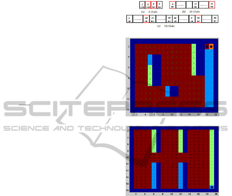
The test domain consists of 5 MDPs as shown in Fig-

ure 3, each with discount factor γ = 0.9. The ﬁrst

three domains are the 4-, 20-, and 50- chain. The 4-,

and 20-domain are also used in (Lagoudakis and Parr,

2003; X. Xu and Lu, 2007) and the 50-chain is used

in (Lagoudakis and Parr, 2003). In general, the x-

open chain which is originally studied in (Koller and

Parr, 2000) consists of a sequence of x states, labeled

from s

to s

. In each state, the agent has 2 actions,

either GoRight (R) or GoLeft (L). The actions suc-

ceed with probability 0.9 changing the state in the in-

tended direction and fail with probability 0.1 chang-

ing the state in the opposite direction. The reward

structure can vary such as the agent gets reward for

visiting the middle states or the end states. For the

4-chain problem, the agent is rewarded 1 in the mid-

dle states, i.e. s

and s

, and 0 at the edge states, i.e.

and s

. The optimal policy is R in states s

and

and L in states s

and s

. (Koller and Parr, 2000)

used a policy iteration method to solve the 4-chain

and showed that the resulting suboptimal policies os-

cillate between R R R R and L L L L. The reason is

because of the limited approximation abilities of basis

functions in policy evaluation. For the 20-chain, the

agent is rewarded 1 in states s

and s

, and 0 else-

OnlineKnowledgeGradientExplorationinanUnknownEnvironment

1. Input:

|S|

;

|A|

;discount factor

;accuracy

;

set of basis functions

Φ = {φ

,···,φ

}

;initial

learned policy

;length of trajectory

;

policy improvement interval

;reward

r ∼ N(µ

,σ

)

; initial state

2. Intialize:

A ←0

;

b ←0

;

Dic

= { }

;

|SA|×|SA|

=< Φ

,Φ >

;

−1

Dic

= []

;

|SA|

← 0

3. For

t = 1, ···, L

← KG

, a

; observe:

t+1

;

t+1

← π

t+1

)

← (s

) ∗|A|+ a

t+1

← (s

t+1

) ∗|A|+ a

t+1

7. For

∈ {z

, z

t+1

}

(.,z

) = [k(1,z

),···,k( j,z

),···,k(|Dic

|, z

)]

c(z

) = K

−1

Dic

∗ k(., z

)

error(z

) = k(z

) −k

(.,z

) ∗ c(z

)

10. If

error(z

) > v

11.

Dic

t+1

← Dic

∪ z

;

−1

Dic

t+1

←

error(z

)



error(z

−1

Dic

−c(z

)

−c(z

)



;

←



0 0



;

←





12. Else

Dic

t+1

← Dic

;

−1

Dic

t+1

← K

−1

Dic

13. End if

14. End for

15.

t+1

←

+ k(.,z

)[k(., z

) −γ k(., z

t+1

)]

16.

t+1

←

+ k(.,z

k(., z

) = [k(1,z

),···,k( j,z

),···,k(|Dic

t+1

|, z

)]

17. If

t = (l + 1)K

then

18.

ˆw

←

−1

t+1

19. for

z = z

, z

, ···, z

|SA|

k(., z) = [k(1, z),···, k( j,z),···, k(|Dic

t+1

|, z)]

(z) = ˆw

∗ k(., z)

end

20.

t+1

← argmax

(s,a)∀

s∈ S

;

← π

t+1

;

l ← l + 1

21. End if

22.

← s

t+1

23. End for

24. Output: At each time step

, note down:

the reward

and the learned policy

Figure 2: Algorithm: (Online-KBLSPI).

where. The optimal policy is L from states s

through

and R from states s

through s

. And, for the

50-chain, The agent gets reward 1 in states s

and

and 0 elsewhere. The optimal policy is R from

state s

through state s

and from state s

through

state s

, and L from state s

through state s

and

from state s

through state s

(Lagoudakis and Parr,

2003). The fourth and ﬁfth MDPs, the grid

and grid

worlds, are used in (Sutton and Barto, 1998). The

agent has 4 actions Go Up, Down, Left and Right and

for each of them it transits to the intended state with

probability 0.7 and fails with probability 0.1 chang-

ing the state to the one of other directions. The agent

gets reward 1 if it reaches the goal state, −1 if it hits

(a) The chain domains

(b) The grid

domain

Figure 3: Subﬁgure (a) is the chain domains, in the red cells,

the agent gets rewards. Subﬁgure (b) is the grid

with 280

states and 188 accessible states. Subﬁgure (c) is the grid

with 400 states and 294 accessible states. The arrows show

the optimal actions in each state.

the wall, and 0 elsewhere.

The experimental setup is as follows: For each of

the 5 MDPs, we compared online-LSPI and online-

KBLSPI using knowledge gradient KG policy as an

exploration policy. For number of experiments EXPs

equals 1000 for the chain domains, 100 for the grid

domain and 50 for the grid

domain, each one with

length L. The performance measures are: 1) the av-

erage frequency at each time step, i.e. at each time

step t for each experiment, we computed the proba-

bility that the learned policy (step: 19) in Algorithm 2

reached to the optimal policy, then we took the aver-

age of EXPs experiments to give us the average fre-

quency at each time step. 2) the average cumulative

ICAART2014-InternationalConferenceonAgentsandArtificialIntelligence

frequency at each time step, i.e. the cumulative aver-

age frequency at each time step t. (Mahadevan, 2008)

used the 50-chain domain with length of trajectories

L equals 5000, therefore, we used the same horizon.

For other MDP domains we adapted the length of tra-

jectories L according to the number of states, i.e. as

the number of states is increased, L will be increased.

For instance, L is set to 18800 for the grid world.

KG policy, needs estimated standard deviationand

estimated mean for each state-action pair. Therefore,

we assume that the reward has a normal distribution.

For example, for the 50-chain problem, the agent is

rewarded 1 if it goes to state 10, therefore, we set the

reward in s

to N(µ

,σ

), where µ

= 1. And, the

agent is rewarded 0 if it goes to s

, therefore, we set

the reward to N(µ

,σ

), where µ

= 0. σ

is the stan-

dard deviation of the reward which is set ﬁxed and

equal for each action, i.e. σ

= 0.01,0.1, 1. More-

over, KG exploration policy is a full optimistic pol-

icy, therefore, we set the policy improvement inter-

val K

to 1. For each run, the initial state s

was

selected uniformly, randomly from the state space S.

We used the pseudo-inversewhen the matrix

A is non-

invertible (Mahadevan, 2008).

For online KBLSPI, we deﬁne a kernel function

K on state-action pairs, i.e. K : |SA|×|SA| → R , we

composed K into a state kernel K

, i.e. K

: |S|×|S|→

R and an action kernel K

, i.e. K

: |A|×|A| → R

as (Y. Engel and Meir, 2005). Therefore, the ker-

nel function K is K = K

⊗K

where ⊗ is the Kro-

necker product. K is a kernel matrix because K

and

are kernel matrices, we refer to (Scholkopf and

Smola, 2002) for more details. The kernel state K

is a Gaussian kernel, i.e. k(s,s

′

) = exp

−||s−s

′

/(2σ

)

where σ

is the standard deviation of the kernel state

function, s is the state at time t and s

′

is the state at

time t+1. And, the action kernel is a Gaussian kernel,

i.e. k(a,a

′

) = exp

−||a−a

′

/(2σ

)

where σ

is the standard

deviation of the kernel action function, a is the action

at time t and a

′

is the action at time t + 1. s and s

′

and a and a

′

are normalized as (X. Xu and Lu, 2007),

e.g. for 50-chain with number of states |S| = 50 and

number of actions |A| = 2, s,s

′

∈ {

/|S|,··· ,

/|S|} and

a,a

′

∈{0.5,1}. σ

and σ

are tuned empirically and

set to 0.55 for the chain domains and 2.25 for the grid

world domains (grid

and grid

) We set the accuracy

v in the approximated kernel basis to 0.0001.

For online-LSPI, we used Gaussian basis func-

tions φ

= exp

−||s−c

/(2σ

)

where φ

is the basis

functions for state s with center nodes (c

)

i=1

which

are set with equal distance between each other, and

is the standard deviation of the basis functions

which is set to 0.55. The number of basis functions

n equals 3 for 4-chain, 5 for 20-chain, and 10 for

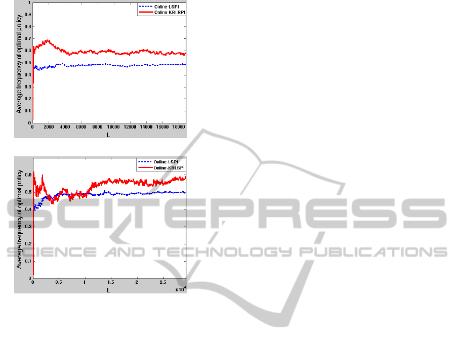
(a) Performance on 4-chain domain

(b) Performance on 20-chain domain

Figure 4: Performance of the average frequency by the KG

policy in online-LSPI in blue and KG in online-KBLSPI in

red. Subﬁgure (a) shows the performance on the 4-chain

using standard deviation of reward σ

= 0.01. Subﬁgure

(b) shows the performance on the 20-chain using standard

deviation of reward σ

= 1. Subﬁgure (c) shows the perfor-

mance on the 50-chain using σ

= 0.1.

50-chain as (Lagoudakis and Parr, 2003) and 40 for

the grid

and grid

domains as (M. Sugiyama and Vi-

jayakumar, 2008).

4.2 Experimental Results

The experimental results on the chain domains, i.e.

4-, 20-, and 50-chain show that the online-KBLSPI

OnlineKnowledgeGradientExplorationinanUnknownEnvironment

(a) Performance on grid

domain

(b) Performance on grid

domain

Figure 5: Performance of the average frequency by the KG

policy in online-LSPI in blue and KG in online-KBLSPI

in red. Subﬁgure (a) shows the performance on the grid

domain using standard deviation of reward σ

= 0.01. Sub-

ﬁgure (b) shows the performance on the grid

domain using

standard deviation of reward σ

= 1.

outperforms the online-LSPI according to the average

frequency and cumulative average frequency of op-

timal policy performances for all values of the stan-

dard deviation of reward σ

i.e. σ

= 0.01, 0.1 and 1.

Figure 4 shows how the performance of the learned

policy is increased by using online-KBLSPI on the 4-

chain, 20-chain and 50-chain.

The experimental results on the grid

domain

show that the online-KBLSPI outperforms the online-

LSPI according to the average frequency and cumu-

lative average frequency of optimal policy perfor-

mances for all values of the standard deviation of

reward σ

i.e. σ

= 0.01,0.1 and 1. And, the ex-

perimental results on the grid

domain show that the

online-KBLSPI performs better than the online-LSPI

for standard deviation of reward equals 1. Figure 5

shows how the performance of the learned policy is

increased by using online-KBLSPI on the grid

and

grid

domains.

The results clearly show that online-KBLSPI usu-

ally converges faster than online-LSPI to the (near)

optimal policies, i.e. the performance of the online

KBLSPI is increased. Although, the performance of

the online LSPI is better in the beginning and this is

because the online LSPI uses its all basis functions,

while online KBLSPI incrementally constructs its ba-

sis functions by the kernel sparsiﬁcation method.

4.3 Statistical Methodology

We used a statistical hypothesis test, i.e. students t-

test with signiﬁcance level α

= 0.05 to compare the

performance of the average frequency of optimal pol-

icy that results from the online-LSPI and the online-

KBLSPI at each time step t. The null hypothesis H

is the online-KBLSPI average frequency performance

(AF

KBLSPI

) larger than the online-LSPI average fre-

quency performance (AF

LSPI

) and the alternative hy-

pothesis H

is AF

KBLSPI

less or equal AF

LSPI

. We

wanted to calculate the conﬁdence in the null hypoth-

esis, therefore, we computed the conﬁdence probabil-

ity p-value at each time step t. The p-value is the

probability that the null hypothesis is correct. The

conﬁdence probability converges to 1 for all standard

deviation of reward, i.e. σ

= 0.01, 0.1, and 1 and for

all domains, i.e. the 4-, 20-, and 50-chain domains

and the grid world domains. Figure 6 shows how

the p-value converges to 1 using the 50-chain, and

the grid

domain with standard deviation of reward

= 0.1. The x-axis gives the time steps (the length

of trajectories). The y-axis gives the conﬁdence prob-

ability, i.e. p-value. Figure 6 shows the conﬁdence

in the online kernel-based LSPI performance is very

high, where the p-value converged quickly to 1.

5 CONCLUSIONS AND FUTURE

WORK

We presented Markov decision process which is a

mathematical model for the reinforcement learning.

We introduced online and ofﬂine least squares policy

iteration (LSPI) that ﬁnd the optimal policy in an un-

known environment. We presented knowledge gradi-

ent KG policy to be used as an exploration policy in

the online learning algorithm. We introduced ofﬂine

kernel-based LSPI (KBLSPI). We also introduced ap-

proximate linear dependency (ALD) method to select

feature automatically and get rid of tuning empirically

the center nodes. We proposed online-KBLSPI which

uses KG exploration policy and ALD method. Fi-

nally, we compared online-KBLSPI and online-LSPI

and concluded that the average frequency of opti-

mal policy performance is improved by using online-

KBLSPI. Future work must compare the performance

ICAART2014-InternationalConferenceonAgentsandArtificialIntelligence

(a) p-value of the 50-chain domain

(b) p-value of the grid domain

Figure 6: The conﬁdence probability p-value that the av-

erage frequency of optimal policy performance of online-

KBLSPI performs better than online-LSPI. Subﬁgure (a)

shows the p-value of the 50-chain using standard deviation

of reward σ

= 0.1. Subﬁgure (b) shows the p-value of the

grid domain using standard deviation of reward σ

= 0.1.

of online-LSPI and online-KBLSPI using other types

of basis functions, e.g. the hybrid shortest path basis

functions (Yahyaa and Manderick, 2012), must com-

pare the performance using continuous MDP domain,

e.g. Interval pendulum and must prove a convergence

analysis of the online-KBLSPI.

REFERENCES

Engel, Y. and Meir, R. (2005). Algorithms and represen-

tations for reinforcement learning. Technical report,

Ph.D. thesis, Senate of the Hebrew.

I.O. Ryzhov, W. P. and Frazier, P. (2012). The knowledge-

gradient policy for a general class of online learning

problems. Operation Research, 60(1):180–195.

Koller, D. and Parr, R. (2000). Policy iteration for fac-

tored mdps. In Proceedings of the 16th Conference

Annual Conference on Uncertainty in Artiﬁcial Intel-

ligence (UAI).

L. Bus¸oniu, D. Ernst, B. D. S. and Babuˇska, R. (2010).

Online least-squares policy iteration for reinforcement

learning control. In Proceedings of the 2010 American

Control Conference.

Lagoudakis, M. G. and Parr, R. (2003). Model-free least

squares policy iteration. Technical report, Ph.D. the-

sis, Duke University.

M. Sugiyama, H. Hachiya, C. T. and Vijayakumar, S.

(2008). Geodesic gaussian kernels for value func-

tion approximation. Journal of Autonomous Robots,

25(3):287–304.

Mahadevan, S. (2008). Representation Discovery Using

Harmonic Analysis. Morgan and Claypool Publish-

ers.

Powell, W. (2007). Approximate Dynamic Programming:

Solving the Curses of Dimensionality. John Wiley and

Sons, New York, USA.

Puterman, M. L. (1994). Markov Decision Processes: Dis-

crete Stochastic Dynamic Programming. John Wiley

and Sons, Inc., New York, USA.

Scholkopf, B. and Smola, A. (2002). Learning with Ker-

nels: Support Vector Machines, Regularization, Opti-

mization, and Beyond. MIT Press, Cambridge, MA,

USA.

Sutton, R. and Barto, A. (1998). Reinforcement Learning:

An Introduction (Adaptive Computation and Machine

Learning). The MIT Press, Cambridge, MA, 1st edi-

tion.

Vapnik, V. (1998). The Grid: Statistical Learning Theory.

Wiley Press, New York, United State of America.

X. Xu, D. H. and Lu, X. (2007). Kernel-based least squares

policy iteration for reinforcement learning. Journal

of IEEE Transactions on Neural Network, 18(4):973–

992.

Y. Engel, S. M. and Meir, R. (2004). The kernel recursive

least-squares algorithm. Journal of IEEE Transactions

on Signal Processing, 52(8):2275–2285.

Y. Engel, S. M. and Meir, R. (2005). Reinforcement learn-

ing with gaussian processes. In Proceedings of the

22nd International Conference on Machine learning

(ICML), New York, NY, USA. ACM.

Yahyaa, S. Q. and Manderick, B. (2012). Shortest path

gaussian kernels for state action graphs: An empirical

study. In The 24th Benelux Conference on Artiﬁcial

Intelligence (BNAIC), Maastricht, The Netherlands.

Yahyaa, S. Q. and Manderick, B. (2013). Knowledge gradi-

ent exploration in online least squares policy iteration.

In The 5th International Conference on Agents and

Artiﬁcial Intelligence (ICAART), Barcelona, Spain.

OnlineKnowledgeGradientExplorationinanUnknownEnvironment