Spontaneous Emission of Radiation by Solitons in Fiber-optic
Waveguides
E. Tchomgo Felenou, P. Tchofo Dinda and C. M. Ngabireng
Laboratoire ICB, UMR CNRS No. 5027, 9 Av. A. Savary, B.P. 47 870, 21078 Dijon C
´
edex, France
Keywords:
Solitons, Pulse Propagation, Radiation Processes, Fiber-optic Waveguide.
Abstract:
We examine the dynamical behavior of light pulses displaying a soliton-like behavior, but which are affected,
when entering a fiber-optic waveguide, by a slight perturbation of profile as compared to the stationary profile
in the waveguide. We show that, surprisingly, certain pulses propagate while emitting a radiation whereas
other pulses emit no radiation. A physical explanation of this difference of behavior is proposed, and tools of
prediction of the radiating or non-radiating character of a light pulse in fiber-optic waveguides, are set up.
1 INTRODUCTION
The soliton, as it was discovered by Zabusky and
Kruskal, (Zabusky and Krukal, 1965), corresponds to
a robust solitary wave that can propagate over large
distances without profile deformation and decrease of
speed. However, over time, the soliton terminology
has acquired different meanings depending on the sci-
entific field in which it is used. In mathematics, the
soliton is an exact solution of some classes of nonlin-
ear equations associated with completely integrable
systems. Obviously, the soliton, as a mathematical
object, corresponds to an idealized representation of
the real world, where the solitary wave propagates
through a perfect physical medium without defects
or perturbations. In fact, real physical systems are
always more or less perturbed (i.e., not totally in-
tegrable), and there, the soliton refers to an energy
packet propagating without significant deformation or
modification of its speed. In the present study, for
sake of simplicity, we use the soliton terminology to
designate all the light pulses displaying a soliton-like
behavior, whether the pulse is affected by a pertur-
bation or not. In this context, it is worth noting that
the presence of small perturbations in a soliton sys-
tem leads to many fundamental effects, such as, an
alteration of the soliton profile as compared to the
stationary profile in the waveguide, or the occurrence
of internal dynamics within the soliton. More impor-
tantly, in certain situations which have never been re-
ally elucidated so far, the perturbed soliton generates
radiation waves, i.e., wave packets of low-amplitude
which follow, or sometimes precede the soliton (Gor-
don, 1992; Remoissenet, 1993; Ngabireng and Dinda,
2005). This radiation phenomenon is incontestably
the most dramatic of the perturbation effects, and also
one of the most detrimental to the pulse stability in
many practical systems, and specifically in long-haul
optical communication systems. In this work, we ex-
amine the dynamical behavior of light pulses which
are affected, when entering a fiber-optic waveguide
(FOWG), by slight distortions of profile as compared
to the stationary profile in the waveguide. In par-
ticular, we address a fundamental question left open
until now. Indeed, until very recently, the idea was
widespread that a perturbed pulse necessarily emits
a radiation. However, this idea has been questioned
in recent studies (Ngabireng and Dinda, 2005), which
demonstrated the existence of non radiating pulses.
However, to our knowledge, no physical explanation
related to the non-radiating behavior of certain light
pulses, has been proposed in the literature so far. In
the present study, we have discovered that the struc-
ture of the pulse profile at the entrance of waveguide,
contains elements that explain surprisingly well, and
even that can predict the presence or the absence of
radiation. Furthermore, we propose theoretical tools
that allow one to clearly identify the radiation waves
and localize exactly their positions in the waveguide.
Those tools constitute the access key to strategies of
suppression of radiation in numerous systems where
this phenomenon is undesirable.
74
Tchomgo Felenou E., Tchofo Dinda P. and Ngabireng C..
Spontaneous Emission of Radiation by Solitons in Fiber-optic Waveguides.
DOI: 10.5220/0004706700740078
In Proceedings of 2nd International Conference on Photonics, Optics and Laser Technology (PHOTOPTICS-2014), pages 74-78
ISBN: 978-989-758-008-6
Copyright
c
 2014 SCITEPRESS (Science and Technology Publications, Lda.)

2 QUALITATIVE AND
QUANTITATIVE
CONSIDERATIONS
As we mentioned above, during their propagation in
a FOWG, light pulses are subject to a perturbed en-
vironment. Perturbations may have two main origins:
They may be induced by the waveguide, i.e., be con-
substantial to the system. Other perturbations can be
external to the system, i.e., related to the action of
an agent external to the system. For sake of clarity
of presentation, we shall discuss separately these two
situations.
2.1 Perturbation Induced by the
Periodic Structure of the Waveguide
As is well known, the conventional optical soliton
is the result of a delicate balance between two ef-
fects that compensate exactly, namely, the self-phase
modulation and the anomalous dispersion of the fiber
(Hasegawa and Tappert, 1973; L. F. Mollenauer and
Gordon, 1980). In a FOWG, as the pulse propagates
through the system, it undergoes losses which gradu-
ally reduce the self-phase modulation. Consequently,
the balance between self-phase modulation and dis-
persion can no longer be maintained in the real sys-
tem. In this context, several alternative strategies have
been developed in order to stabilize pulse propaga-
tion in FOWGs, leading to the emergence of partic-
ularly robust pulses such as the guiding-center soli-
ton (GCS) or the dispersion-managed soliton, which
are able to propagate in a highly stable manner over
several thousands of kilometers. All of those strate-
gies have as common general feature, the fact of be-
ing based on periodically structured waveguides, i.e.,
which are made up of the repetition of the same ba-
sic structure called amplification span. Within each
span, the pulse executes a relatively fast internal dy-
namics, before going back (at the end of the span)
to a profile identical or close to the one it was hav-
ing at the beginning of the span. Most of the periodi-
cally structured waveguides, admit stationary pulses.
Here, the terminology of stationary pulse (SP) refers
to a pulse that propagates while executing, in a pe-
riodic manner, a deformation of profile whose peri-
odicity corresponds exactly to that of the waveguide
(say, Z
A
). If one disregards the internal dynamics
within each amplification span (i.e., the fast dynamic
induced by the combined actions of the exponential
attenuation of the pulse peak power, the dispersion,
and the amplification process), and if one considers
only the pulse profile at the end of each span (slow
dynamic), then the SP will display a behavior identi-
cal to that of a conventional soliton (i.e., a propagation
without change of profile). However, at this juncture,
we wish to point out a crucial point. Indeed, there is
a major qualitative difference between the ideal sys-
tem, where the (conventional) soliton propagates with
a perfectly smooth profile (of Sech shape), and the pe-
riodically structured waveguides, where the profile of
the SP is never smooth. In fact, the internal dynamic
of the pulse, which is closely related to the structure
of the amplification span, significantly alters the pro-
file of the SP, which becomes rough. To illustrate the
perturbation induced by the waveguide on the pro-
file of SPs, we will use a waveguide corresponding
to a GCS (guiding-center soliton) (Hasegawa and Ko-
dama, 1990). In this waveguide the amplification span
consists of only one section of fiber with anomalous
dispersion, followed by an amplifier. The choice of
this waveguide is dictated only by a concern of sim-
plicity, and does not restrict in any way the generality
of the tools that we will develop afterward. Note that
the technique of GCS is based on the compensation
of dispersion by the self-phase modulation, but not in
an instantaneous way. Indeed, as the self-phase mod-
ulation decreases gradually as the pulse propagates
along the amplification span, the pulse is initially en-
dowed with a peak power P
0
larger than that of the
conventional soliton in the same waveguide (say, P
m
),
so that in the beginning of the span, the nonlinearity is
stronger than the dispersion, and that, afterwards, the
situation gets reversed within the span. So, the power
P
0
is chosen so that the balance between the two ef-
fects is thus globally reached at the end of each ampli-
fication span. In this waveguide, the pulse dynamics
may be described by the generalized generalized non-
linear equation (NLSE) which follows
A
z
= −i
β
2
(z)
2
A
tt
+ iγ
|
A
|
2
A −
α
2
A
+

√
G −1

×
N
∑
n=1
δ(z −nZ
A
)A, (1)
where A refers to the electric field of the pulse, β
2
,
γ and α designate the dispersion, non-linearity, and
linear-attenuation coefficients, respectively. The pa-
rameter G = exp(αZ
A
) refers to the gain of each
amplifier. Here, it is worth noting that in the lit-
erature, there exists no exact analytical expression
for the profiles of SPs in FOWGs. Consequently,
the profiles of SPs in real waveguides are accessi-
ble only numerically, by means of specialized tech-
niques. By following the procedure of Ref.(J. H.
B. Nijhof and knox, 1997), we have obtained the re-
sults depicted in figures 1, for the following typical
parameters: α = 0.24dB/km, D = 1ps/nm/km, β
2
=
SpontaneousEmissionofRadiationbySolitonsinFiber-opticWaveguides
75

−13 ×10
−4
ps
2
/m, ∆T = 2T
0
ln(1 +
√
2) = 40ps, γ =
0.002W
−1
m
−1
, P
m
= 1.2mW , Z
A
= 50km. Here ∆T
corresponds to the temporal width of the pulse. Fig-
ures 1 show the profile of the SP in this waveguide
(solid curve), as well as the profiles of the Gaussian
and Sech pulses closest to the SP. One can observe
that the temporal and spectral profiles of the SP are
not smooth. In particular, the roughness of the station-
ary profile is clearly visible far from the central part
of the SP. However, we will show below that some as-
perities are also present in the central part of the pulse,
but they are more clearly perceptible through the pro-
files of the perturbation fields. Thus, figures 1 demon-
−400 −200 0 200 400
10
−10
10
−1
Time [ps]
|A| [a.u]
−0.1 −0.05 0 0.05 0.1
10
−10
10
0
Frequency [THz]
|A| [a.u]
~
SP
GCS
GP
GP
2
2
HSP
1
1
(a)
(b)
Figure 1: Profile of the stationary pulse (SP), and profiles of
the Gaussian pulse (GP) and Hyperbolic secant pulse (HSP)
closest to the SP.
strate that the GCS proposed in Ref. (Hasegawa and
Kodama, 1990), as well as the Gaussian and Sech
pulses, in spite of their exceptional robustness, do not
correspond rigorously to SPs in the waveguide, be-
cause of their smooth profiles. Here we have used
the GCS whose profile between two consecutive am-
plifiers Z
n
A
and Z
n+1
A
, is given by (Hasegawa and Ko-
dama, 1990):
A
GCS
(z,t) = V
0
√
P
m
exp
h
−
α
2
(z −Z
n
A
)
i
sech

t
T
0

×exp

i
z
2Z
C

, (2)
where V
0
is the enhancement factor of the input peak
power, P
m
is the average power of pulse over the am-
plification span, and Z
C
=T
2
0
/
|
β
2
|
=1/γP
m
. One of the
most outstanding results in figure 1(b), is the presence
of several pairs of sidebands (indicated by numbered
labels), which constitute the most clear distinguish-
ing mark of the waveguide effects on the profile of
the SP. These sidebands, which are sometime called
Kelly bands (Kelly, 1992), result from a process in
which two photons of the soliton, of frequency ω
0
,
are destroyed simultaneously to create two new pho-
tons at frequencies ω
0
−Ω and ω
0
+ Ω. This pro-
cess satisfies the following phase-matching condition:
2k
0
= k
s
+ k
a
+ 2k
I
where k
I
=
2πp
Z
A
represents the
wave vector corresponding to the harmonic of order
p of the oscillation of the pulse peak power, while
k
s
, k
a
and k
0
are respectively the Stokes, anti-Stokes,
and soliton wave vectors. One can easily obtain the
sideband frequencies that fulfill the phase-matching
condition:
Ω
p
= ±
s
1
|
β
2
|

4πp
Z
A
−
1
Z
C

(3)
The frequencies (3) coincide perfectly with those of
the sidebands in figure 1 (b). Thus, the presence of
Kelly bands constitutes one of the most dramatic per-
turbation effects induced by the waveguide on the pro-
file of the SPs. The growth of Kelly bands is system-
atically accompanied by a specific radiation.
2.2 External Perturbation to the System
The complexity of the profile of SPs in FOWG, is
detrimental to the development of those waveguides,
because complexes profiles of light pulses are not fea-
sible with currently available optical devices. In prac-
tice, for a better stability of the pulse propagation in
the waveguide, one endeavors to make so that the in-
put pulse, say A(0,t), is as close as possible to the SP
A
S
(0,t), At this juncture, it is crucial to realize that
the injection of the field A(0,t), which is different but
very close to A
S
(0,t), is felt by the waveguide as a
perturbation of the SP, by a perturbation field q(0,t)
such as:
q = A −A
S
, (4)
where |q(0,t)|  |A
S
(0,t)|, In other words, every-
thing happens as if, when entering the waveguide the
SP A
S
(0,t) collides with the perturbation q(0,t). We
show below that, in fact, the input profile of the per-
turbation field q(0,t) contains a set of special signs
allowing the prediction of the general dynamical be-
havior of the pulse, and specifically, the prediction of
the radiating and non-radiating character of the pulse.
PHOTOPTICS2014-InternationalConferenceonPhotonics,OpticsandLaserTechnology
76

Once the stationary profile of the pulse is known, and
if we have a pulse that fits at best to this stationary
profile, then one can easily obtain the input profile of
the perturbation field. Thus, if we choose to propagate
Gaussian or Sech pulses [A
g
(0,t) or A
sech
(0,t)] that fit
at best to A
S
(0,t), we can then deduce the correspond-
ing perturbation fields, q
g
(0,t) = A
g
(0,t) −A
S
(0,t)
and q
sech
(0,t) = A
sech
(0,t) −A
S
(0,t), associated with
A
g
(0,t) and A
sech
(0,t), respectively. The perturbation
field for the GCS is given by q
GCS
(0,t) = A
GCS
(0,t)−
A
S
(0,t).
−400 −200 0 200 400
10
−7
10
−3
(a1)
|q| [a.u]
−0.1 0 0.1
10
−10
10
−1
~
(b1)
|q| [a.u]
−400 −200 0 200 400
10
−7
10
−3
(a2)
|q| [a.u]
−0.1 0 0.1
10
−10
10
−1
~
(b2)
|q| [a.u]
−400 −200 0 200 400
10
−7
10
−3
(a3)
|q| [a.u]
−0.1 0 0.1
10
−10
10
−1
~
(b3)
|q| [a.u]
4T
Sech
4T
Gauss
Frequency [THz]
Time [ps]
T
GCS
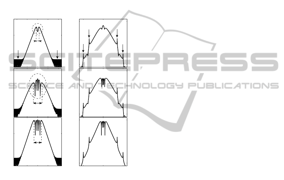
Figure 2: Plot of the perturbation fields associated to the
GCS [(a1) and (b1)], the Sech pulse [(a2) and (b2)], and
Gaussian pulse [(a3) and (b3)] closest to the SP.
Figures 2 show the temporal and spectral profiles of
the perturbation fields, for the three types of pulses
under consideration. In particular, the temporal pro-
files of those perturbation fields exhibit an oscillatory
structure [surrounded by the dashed lines in figures
2(a1) and 2(a2)], which is an indication of the rough-
ness of the central part of the SP profile. More impor-
tantly, a careful inspection of this oscillatory struc-
ture, has enabled us to set up a procedure for the iden-
tification of the radiating or non-radiating character of
the pulse. Indeed, we have found that the pulse is ca-
pable of generating sidebands of radiation only if this
oscillatory structure contains a minimum of full peri-
ods of oscillations, of the order of four periods. Thus,
as figure 2 (a1) shows, the oscillatory structure for
the perturbation field associated with the GCS, con-
tains only a single period of oscillation. We predict
that this pulse will be unable to generate sidebands
of radiation. Quite in contrast, as figures 2(a2) and
2(a3) show, the perturbation fields associated with the
Sech and Gaussian pulses, are endowed with four full
periods of oscillation; which is largely sufficient to
activate a spectral reorganization leading to the gen-
eration of sidebands of radiation. We then predict that
the Sech and Gaussian pulses belong to the category
of radiating solitons. In general, we have discovered
that the central part of the perturbation field always
contains an oscillatory structure which constitutes the
germ of an eventual radiation process in the FOWG.
The more the size of this germ is big, the more the
capacity of radiation of the pulse is high. This obser-
vation is the most important result of our study. By
the way, it is worth noting that the Kelly bands are
also clearly visible in the spectra of the perturbation
fields q(0,t) [see Figs 2(b1), 2(b2), and 2(b3)].
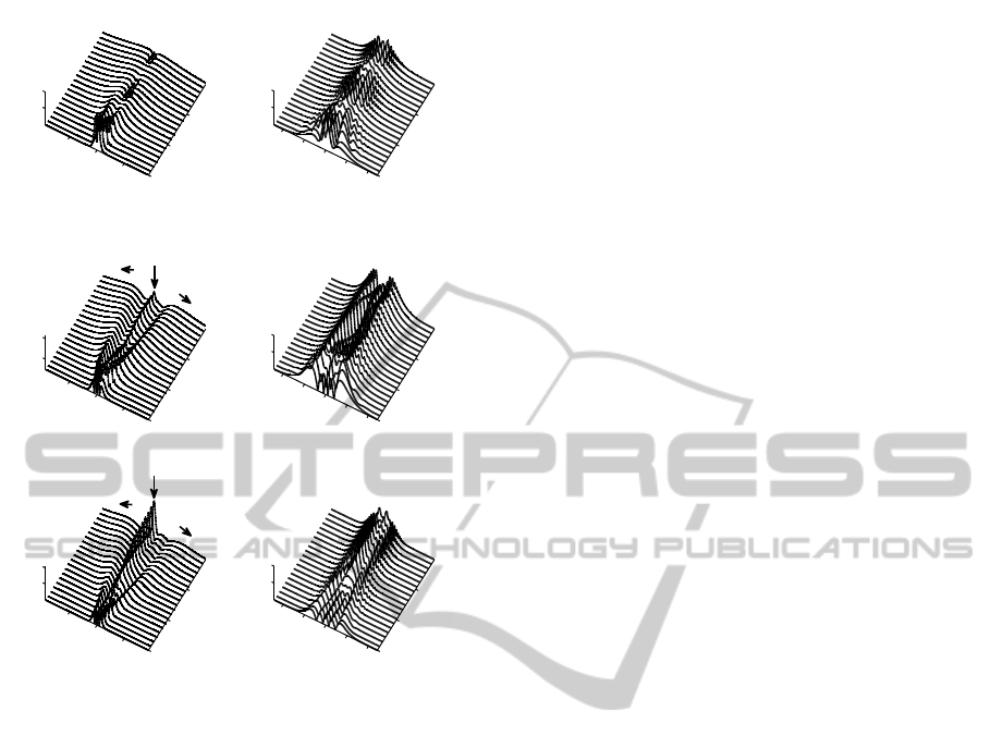
The above predictive analysis is remarkably con-
firmed by the numerical simulations of propagation of
the considered pulses. Figures 3 (a1) - (b1), which
show the evolution of the perturbation field associ-
ated with the propagation of the GCS over a distance
of 6000km, confirms our prediction on the absence
of radiation. We can clearly observe in figure 3(a1),
which results from the propagation of the GCS, that
the pulse executes a restructuration of profile, which
results in a progressive modification of the perturba-
tion field. But the spectral restructuration of the pulse
is not sufficient to activate the process of radiation [as
shown in figure 3(b1)]. One can finally observe in
figure 3(a1) that the pulse absorbs the perturbation,
but without being able to contain it over all the prop-
agation distance. Consequently, the perturbation field
widens continually (while flattening) during the prop-
agation. Figures 3 (a2)-(b2), which show the evolu-
tion of the perturbation field associated with the prop-
agation of the pulse having initially a Sech profile,
confirm our prediction on the existence of a radiation
process. The temporal profile of the perturbation field
in figure 3 (a2), shows clearly two waves of radia-
tion moving away from the center of the pulse rest
frame. At the center of this frame, one can clearly
distinguish a trapped field (corresponding to the non
radiating part of the perturbation field). Figures 3(a3)-
(b3) show that injection of the Gaussian pulse leads
to a behavior qualitatively similar to that of the Sech
pulse in figures 3 (a2)-(b2), namely, the radiation of a
part of the perturbation and the trapping of the other
part. We have noticed only a quantitative difference
in the amplitude of the trapped field, which is higher
in the case of the Gaussian pulse.
SpontaneousEmissionofRadiationbySolitonsinFiber-opticWaveguides
77

0
2
4
−500
0
500
0.3
0.6
Z [Mm]
(a1)
Time [ps]
|q| [mW
1/2
]
0
2
4
−0.04
−0.02
0
0.02
0.04
0.5
1
Z [Mm]
(b1)
Frequency [Thz]
|q| [a.u]
~
0
2
4
−500
0
500
0.1
0.3
Z [Mm]
(a2)
Time [ps]
|q| [mW
1/2
]
0
2
4
−0.04
−0.02
0
0.02
0.04
0.5
1
Z [Mm]
(b2)
Frequency [Thz]
|q| [a.u]
~
0
2
4
−500
0
500
4
8
Z [Mm]
(a3)
Time [ps]
|q| [mW
1/2
]
0
2
4
−0.04
−0.02
0
0.02
0.04
0.5
1
Z [Mm]
(b3)
Frequency [Thz]
|q| [a.u]
~
Figure 3: Propagation of the perturbation fields generated
by the guiding-center soliton [(a1) and (b1)], the hyperbolic
secant closest to the SP [(a2) and (b2)], and the Gaussian
profile closest to the SP [(a3) and (b3)]. In figures (a2) and
(a3) the horizontal arrows indicate the radiated waves. The
vertical arrow indicates the part of the perturbation which is
trapped within the pulse.
3 CONCLUSIONS
We have examined the dynamical behavior of a light
pulse near its stationary state, and in particular, the
physical processes that generate radiation waves. It
emerges from our analysis that a light pulse (endowed
with a non-stationary profile in the waveguide), al-
ways executes a restructuration of profile in order to
get closer to the stationary profile. It is during this
process of restructuration of profile that certain pulses
emit a radiation while other pulses emit no radiation.
We have shown that the ability to radiation is deter-
mined by the initial structure of the perturbation field,
defined as the disagreement of profile between the in-
put pulse and the SP in the waveguide. We have estab-
lished the existence of an oscillatory structure in the
central part of the perturbation field, whose size de-
termines the ability to radiate. Non-radiating pulses
are characterized by an oscillatory structure contain-
ing only a few periods of oscillation (typically, less
than four periods of oscillation). Radiating pulses
are characterized by an oscillatory structure contain-
ing a large number of periods of oscillation (typically,
at least four periods of oscillation). Finally, the fact
that we can clearly identify the radiation and local-
ize exactly its position in the waveguide, leads us to
consider its suppression as feasible in certain prac-
tical systems where this phenonema is undesirable,
such as in long-haul optical communication systems,
or mode-locked fiber lasers.
ACKNOWLEDGEMENTS
E. Tchomgo Felenou acknowledges the SCAC (Ser-
vice de Coop
´
eration et d’Action Culturelle) for his fi-
nancial support.
REFERENCES
Gordon, J. P. (1992). Dispersive pertubations of solitons
of non linear schdinger equation. J. Opt. Soc. Am. B,
9:91–97.
Hasegawa, A. and Kodama, Y. (1990). Guiding-center soli-
ton in optical fibers. Opt. Lett., 15:1443–1445.
Hasegawa, A. and Tappert, F. (1973). Transmission of sta-
tionary nonlinear optical pulses in dispersive dielec-
tric fibers. i. anomalous dispersion. Appl. Phys. Lett.,
23:142–144.
J. H. B. Nijhof, N. J. Doran, W. F. and knox, F. M. (1997).
Stable soliton-like propagation in dispersion managed
systems wiyh net anomalous, zero and normal disper-
sion. Electron Lett., 33:1726–1727.
Kelly, S. M. (1992). Characteristic sideband instability of
periodically amplified average soliton. Electron. Lett.,
28:806–807.
L. F. Mollenauer, R. H. S. and Gordon, J. P. (1980). Experi-
mental observation of picosecond pulse narrowing and
solitons in optical fibers. Phys. Rev. Lett., 45:1095–
1098.
Ngabireng, C. M. and Dinda, P. T. (2005). Radiating and
non-radiating dispersion-managed solitons. Opt. Lett.,
30:595–597.
Remoissenet, M. (1993). Waves called solitons: concepts
and experiments. 3rd ed., Springer-Verlag, Berlin Hei-
delberg.
Zabusky, N. J. and Krukal, M. D. (1965). Interaction of
solitons in a collisionless plasma and the recurrence
of initial states. Phys. Rev. Lett., 15:240–243.
PHOTOPTICS2014-InternationalConferenceonPhotonics,OpticsandLaserTechnology
78