Active Shape Models with SIFT Descriptors and MARS

Stephen Milborrow and Fred Nicolls

Department of Electrical Engineering, University of Cape Town, Cape Town, South Africa

Keywords:

Facial Landmark, Active Shape Model, Multivariate Adaptive Regression Splines.

Abstract:

We present a technique for locating landmarks in images of human faces. We replace the 1D gradient pro-

ﬁles of the classical Active Shape Model (ASM) (Cootes and Taylor, 1993) with a simpliﬁed form of SIFT

descriptors (Lowe, 2004), and use Multivariate Adaptive Regression Splines (MARS) (Friedman, 1991) for

descriptor matching. This modiﬁed ASM is fast and performs well against existing techniques for automatic

face landmarking on frontal faces.

1 INTRODUCTION

In this paper we use the Active Shape Model (ASM)

of (Cootes et al., 1995) for locating facial land-

marks, but use a simpliﬁed form of SIFT (Lowe,

2004) descriptors for template matching, replacing

the 1D proﬁles used in the classical model. Ad-

ditionally, we use Multivariate Adaptive Regression

Splines (MARS) (Friedman, 1991) to to efﬁciently

match these descriptors around the landmark. We also

introduce techniques for signiﬁcantly decreasing their

computational load, making SIFT based ASMs use-

able in practical applications.

First a brief overview of ASMs. For details

see (Cootes and Taylor, 2004). A landmark represents

a distinguishable point present in most of the images

under consideration, for example the nose tip (Fig-

ure 1). A set of landmarks forms a face shape. The

ASM starts the search for landmarks from the mean

Figure 1: A landmarked face (Milborrow et al., 2010).

training face shape aligned to the position and size of

the image face determined by a global face detector.

It then repeats the following two steps until conver-

gence:

(i) Suggest a new shape by adjusting the current

positions of the landmarks. To do this at each land-

mark it samples image patches in the neighborhood of

the landmark’s current position. The landmark is then

moved to the center of the patch which best matches

the landmark’s model descriptor. (The landmark’s

model descriptor is generated during model training

prior to the search.)

(ii) Conform the suggested shape to a global

shape model. This pools the results of the individ-

ual matchers and corrects points that are obviously

mispositioned. The shape model is necessary because

each matcher sees only a small portion of the face and

cannot be completely reliable (Figure 2).

The entire search is repeated at each level in an im-

age pyramid, typically four levels from coarse to ﬁne

resolution. In this paper our focus is on step (i), the

template matching step. We leave step (ii) unchanged.

Figure 2: 15 × 15 patches of the nose tip in Figure 1. The

left patch is at half image scale; the right is at full scale.

380

Milborrow S. and Nicolls F..

Active Shape Models with SIFT Descriptors and MARS.

DOI: 10.5220/0004680003800387

In Proceedings of the 9th International Conference on Computer Vision Theory and Applications (VISAPP-2014), pages 380-387

ISBN: 978-989-758-004-8

 2014 SCITEPRESS (Science and Technology Publications, Lda.)

2 RELATED WORK

Numerous proposals have been made to replace the

1D proﬁles of the classical ASM. We mention just a

few SIFT based schemes, emphasizing facial applica-

tions. (Zhou et al., 2009) use SIFT descriptors with

Mahalanobis distances. They report improved eye

and mouth positions on the FGRCv2.0 database. (Li

et al., 2009) use SIFT descriptors with GentleBoost.

(Kanaujia and Metaxas, 2007) use SIFT descriptors

with multiple shape models clustered on different face

poses. (Belhumeur et al., 2011) use SIFT descriptors

with SVMs and RANSAC. They report excellent ﬁts,

albeit at speeds orders of magnitude slower than ours.

(Shi and Shen, 2008) use SIFT descriptors in hier-

archical ASM models for medical images. SIFT de-

scriptors for face data are also used in (Querini and

Italiano, 2012; Rattani et al., 2007; Zhang and Chen,

2008; Zhang et al., 2011).

Multivariate Adaptive Regression Splines

(MARS) is a general purpose regression technique

introduced by Jerome Friedman in a 1990 pa-

per (Friedman, 1991). MARS has been shown to

perform well in diverse applications e.g. (Leathwick

et al., 2005; Vogel et al., 2010), although it is

apparently not well known in the image processing

community. For our purposes the principal advantage

of MARS over related nonparametric regression

methods like SVMs is its prediction speed. Also

making it attractive are short training times and

interpretability of the models it creates

3 SIFT DESCRIPTORS

A descriptor for template matching captures some dis-

tinguishing quality of the image feature in question.

In the ASM context, we want descriptors to capture

the nature of say the inner corner of the left eye. A

simple example is the “gradient descriptor”, which

takes the form of an array with the same dimensions

as the image patch; each element of the array is the

gradient or gradient magnitude at the corresponding

pixel in the patch. Typically the descriptor is normal-

ized to unit length. The classical ASM uses 1D gradi-

ent descriptors. Gradients are invariant to afﬁne light-

ing changes, but not to other changes, so researchers

have devised more sophisticated techniques.

In this section we give an overview of the SIFT

descriptors which form the basis of the “HAT” de-

scriptors used in our version of the ASM. The next

section will then describe how HAT descriptors dif-

fer from SIFTs. We chose SIFT descriptors for in-

vestigation because of their well known good sensi-

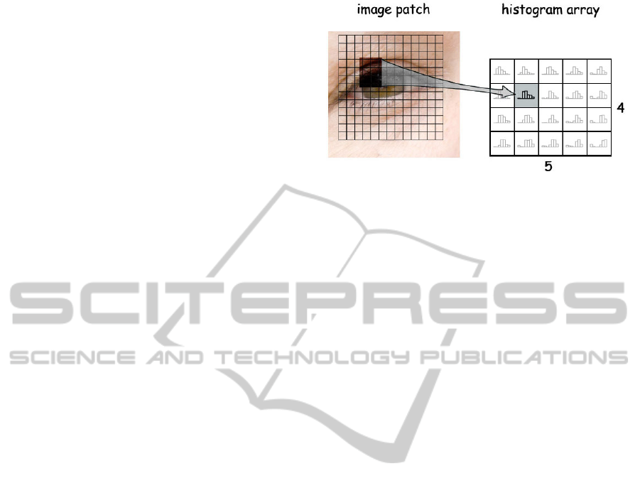
Figure 3: An area in the patch maps to a cell in the his-

togram array.

tivity and speciﬁcity properties. Details can be found

in David Lowe’s paper (Lowe, 2004). Precedents for

the orientation histograms used in SIFT can be found

in e.g. (Belongie et al., 2002; Freeman and Roth,

1995).

The SIFT descriptor takes the form of an array of

histograms (Figure 3). The descriptor is generated

from a rectangular patch around the image point of in-

terest. Ignoring interpolation for now, coordinates in

the patch map to cells in the histogram array. We use a

15 × 15 patch and an array of 4 × 5 histograms. These

dimensions were determined during our ASM train-

ing; other values are also in common use. The low

spatial resolution of the histogram array helps provide

immunity to small changes within the patch while still

picking up overall structure.

Each histogram describes the distribution of gra-

dient orientations in its region of the patch. We use

8 bins per histogram, thus 360/8 = 45 degrees per

bin. The gradient magnitude at a pixel is added to the

histogram bin designated for its orientation, down-

weighted for smoothness by the Gaussian distance

of the pixel from the center of the patch. The ar-

ray of histograms is stored internally as a vector with

4 × 5 × 8 = 160 elements.

In the non-interpolated setup just described, a

small change in the patch position may cause a large

change to the descriptor as the mapping for a pixel

jumps abruptly from one histogram to another. We

thus linearly interpolate, or “smear out”, a pixel’s

contribution across adjacent histograms. The contri-

bution of a pixel which maps to the border between

histogram cells is divided equally between the his-

tograms. A pixel which maps to the center of a cell

affects only the histogram in that cell.

Likewise a small change in the orientation at a

pixel can cause an abrupt jump in assignment from

one histogram bin to another. We therefore also inter-

polate orientations across histogram bins. A gradient

with a 45

◦

orientation is shared equally between the

ActiveShapeModelswithSIFTDescriptorsandMARS

381

bin for 0−45

◦

and the bin for 45−90

◦

Our tests veriﬁed that the Gaussian spatial down-

weighting and all three interpolations (horizontally

and vertically across histograms, and across bins

within a histogram) are necessary for optimum ﬁts in

ASMs, although computationally demanding.

Finally, we take the square root of each element of

the descriptor vector and normalize the resulting vec-

tor to unit length. Taking the square root reduces the

effect of extreme values such as the bright spots on the

nose tip in Figure 1. Normalizing to unit length gives

invariance to linear changes in image contrast. (In-

variance to the absolute illumination level is already

achieved because we are using gradients not gray lev-

els.) Actually, taking the square root is what we use

in our ASM; SIFT descriptors in their original form

use a slightly more complicated scheme.

4 HAT DESCRIPTORS

This section presents the descriptors used in our

model. They are essentially unrotated SIFT descrip-

tors with a ﬁxed scale. In this paper it is convenient to

use the term Histogram Array Transforms (HATs) for

these descriptors.

HAT descriptors can be generated much more

quickly than descriptors in the standard SIFT frame-

work. Speed is important because to locate the land-

marks in a face we need to evaluate something like

25 thousand descriptors. (Using typical parameters:

68 landmarks × 4 pyramid levels × 4 model itera-

tions × 5 × 5 search grid = 27k.)

4.1 No Automatic Scale Determination

Readers familiar with SIFT will be aware that the

overview of descriptors in Section 3 does not mention

the overall SIFT framework in which the descriptors

are used (Lowe, 2004). This framework ﬁrst does a

time consuming scale-space analysis of the image to

discover which points in the image are “keypoints”.

It also discovers the intrinsic scale of each of these

keypoints.

In contrast, in ASMs the keypoints are pre-

determined — they are the facial landmarks — and

the face is prescaled to a constant size before the ASM

search begins. (Our implementation scales to an eye-

mouth distance of 100 pixels.) Thus we do not need

SIFTs automatic determination of scale. The ASM

descriptor patches are a ﬁxed size. The ASM uses a

simple 4 octave image pyramid and the search pro-

ceeds one pyramid level at a time. SIFT’s sub-octave

DOG pyramid where multiple levels are analyzed si-

multaneously is unnecessary.

4.2 No Patch Orientation

In the SIFT framework once the intrinsic scale of a

descriptor has been determined there is an additional

preprocessing step (omitted in Section 3): the local

structure of the image around the point of interest is

analyzed to determine the predominant gradient ori-

entation, and the descriptor is formed from a patch

rotated to this direction. The orientation is computed

by looking for peaks in an orientation histogram (in-

dependent of the histograms in the descriptor array).

In our ASM, however, before the search begins

we rotate the entire image so the eyes are horizon-

tal (after locating the eyes with the OpenCV eye de-

tectors (Castrill

on Santana et al., 2007)). Thus the

automatic orientation described in the previous para-

graph is unnecessary, and in our experiments actually

reduced the quality of ﬁt. We also found it unneces-

sary to orientate the descriptors to the shape bound-

ary as is often done in ASMs. Some rotational varia-

tion will still remain (not every face is the same, and

the eye detectors sometime give false positives on the

eyebrows or fail to ﬁnd eyes, causing mis-positioning

of the ASM start shape), and so we must also rely on

the intrinsic invariance properties of the descriptors.

4.3 Precalculation of Mapping from

Patch to Histogram Array

When generating a SIFT or HAT descriptor, each

pixel in the patch must be mapped to a position in the

array of histograms. Calculating this mapping takes

time, especially for scaled and rotated patches, and

must be done each time we generate a descriptor.

But HATs do not use such scaling or rotation, and

the mapping therefore depends only on the histogram

array dimensions (4 × 5) and the image patch width

(15 pixels), which remain constant through the ASM

search. Thus we can precalculate the mapping indices

just once for all descriptors (or once per pyramid level

if we use different patch sizes at different pyramid lev-

els). In our software this precalculation reduced total

ASM search times by 40%.

4.4 Descriptor Caching

In an ASM search we repeatedly revisit the same im-

age coordinates while iterating the models. Addi-

tionally, at coarse pyramid levels the search areas of

nearby points overlap. We therefore save HAT de-

scriptors for reuse. In practice we get a cache hit rate

VISAPP2014-InternationalConferenceonComputerVisionTheoryandApplications

382

of over 65% (over 65% of the requests for a descriptor

can be satisﬁed by using a saved descriptor). Caching

reduces search time by a further 70%.

5 DESCRIPTOR MATCHING

METHODS

Once we have the descriptor of an image patch, we

need a measure of how well the descriptor matches

the facial feature of interest. This section reviews

some standard techniques for descriptor matching,

leading to the MARS models used in our ASM. (Note

that at each landmark the ASM looks only for the sin-

gle best match in the search region, and so we need

be concerned only with the relative quality of match.)

A simple approach is to take the Euclidean dis-

tance between the descriptor and the mean training

descriptor for the landmark in question. This gives

every histogram bin equal weight, but that is inappro-

priate because pixels on certain edges will be more

important than pixels elsewhere. Furthermore, a high

variance bin is likely to add more noise than informa-

tion.

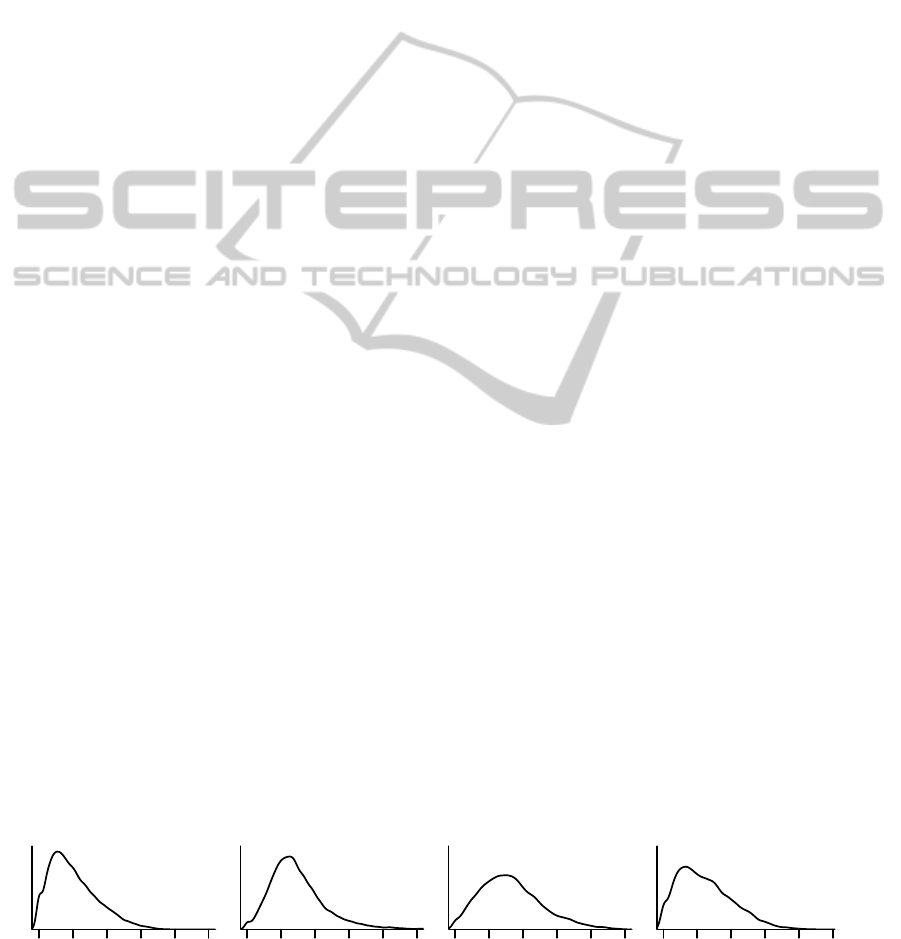
The Mahalanobis distance gives more important

bins more weight (it considers a bin important if it has

low variance in the training set), and takes into con-

sideration interaction between bins. The Mahalanobis

distance is the optimal measure to the extent that the

distribution of the bins’ values is Gaussian, which is

at most only approximately true for count data like

histogram bins (Figure 4). Calculating the Maha-

lanobis distance is slow (proportional to the square of

the number of elements in the descriptor; in our case

160 × 160 = 26k).

Within the standard SIFT framework for key-

point matching, descriptors are matched using near-

est neighbors, but that would be very slow for ASMs,

and for all landmarks would require a large amount of

memory.

Another tack is regression, using sample descrip-

tors on and around the correct position of the land-

marks in training images to train a model that es-

timates match quality as a function of the elements

of the descriptor. Linear regression would be a ﬁrst

choice, but this assumes that the effect of a bin on

the match is proportional to its value, and a straight-

forward application of linear regression makes the as-

sumption that it is unnecessary to account for interac-

tions between bins. These assumptions may be sim-

plistic given that we are looking for a pattern of pixels.

To test that there is enough data to make more com-

plicated regression assumptions, we trained Support

Vector Machines (SVMs) for matching HAT descrip-

tors, which did indeed outperform the other methods

mentioned above. However, SVMs are slow. At each

landmark the SVM after training typically has over a

thousand support vectors. To evaluate a descriptor we

have to take the dot product of the descriptor vector

with each of these vectors (160 × say 1000 = 160k

operations).

We thus turned to Multivariate Adaptive Re-

gression Spline (MARS) models (Friedman, 1991).

MARS models give ASM results that are almost as

good as SVMs and are much faster. In our software,

MARS decreased total search time by over 80%. An

overview of MARS will be given in the next section.

We mention also that in our tests linear SVMs

gave slightly worse ﬁts than the RBF SVMs we used

above. Random Forests (Breiman, 2001) gave not

quite as good ﬁts and took roughly the same time (but

we did not do extensive tuning of Random Forests).

Single CART style trees (Breiman et al., 1984) did

not give good ﬁts.

We generated regression training data as follows.

This regimen was reached after some experimentation

but we do not claim it is optimal. At the landmark of

interest in each training face, we generated (i) three

negative training descriptors at x and y positions ran-

domly displaced by 1 to 6 pixels from the “true” (i.e.,

manually landmarked) position of the landmark, and

(ii) a positive training descriptor at the true position of

the landmark. To bypass issues with imbalanced data,

we duplicated this positive descriptor thrice so there

were equal numbers of positive and negative training

descriptors. We regressed on this data with the posi-

tive training descriptors labeled with 0 and the nega-

tive training descriptors all labeled with 1 irrespective

of their distance from the true position of the land-

0.0 0.5 1.0 1.5 2.0 2.5

bin 5

(hist 0 bin 5)

0.0 0.5 1.0 1.5 2.0 2.5

bin 10

(hist 1 bin 2)

0.0 0.5 1.0 1.5 2.0 2.5

bin 12

(hist 1 bin 4)

0.0 0.5 1.0 1.5 2.0 2.5

bin 13

(hist 1 bin 5)

Figure 4: Non-Gaussianity is evident in the distribution of values across the training set in example histogram bins. Without

the square root mentioned in Section 3, these would be even more non-Gaussian (the square root pulls in the long right tail).

These examples are for the bottom left eyelid in the full scale image.

ActiveShapeModelswithSIFTDescriptorsandMARS

383

mark.

6 MARS

We give a brief overview of MARS by way of

an example. The MARS formula to estimate the

descriptor match at the bottom left eyelid in the full

scale image is

match = 0.026 (1)

+ 0.095 max(0, 1.514 − b

) (2)

+ 0.111 max(0, 2.092 − b

) (3)

+ 0.258 max(0, b

− 1.255) (4)

− 0.108 max(0, 1.574 − b

) (5)

· · · (6)

where the b

are HAT descriptor bins 0 ...159. There

happen to be 17 terms in the formula; we have shown

just the ﬁrst few. The MARS model building algo-

rithm generated the formula from the training data.

There is a similar formula for each landmark at each

pyramid level.

The bins enter the formula via the max functions

rather than directly as they would in a linear model.

The max functions are characteristic of MARS. They

allow nonlinear dependence on the value of a bin and

contain the effect of a bin to a range of its values. The

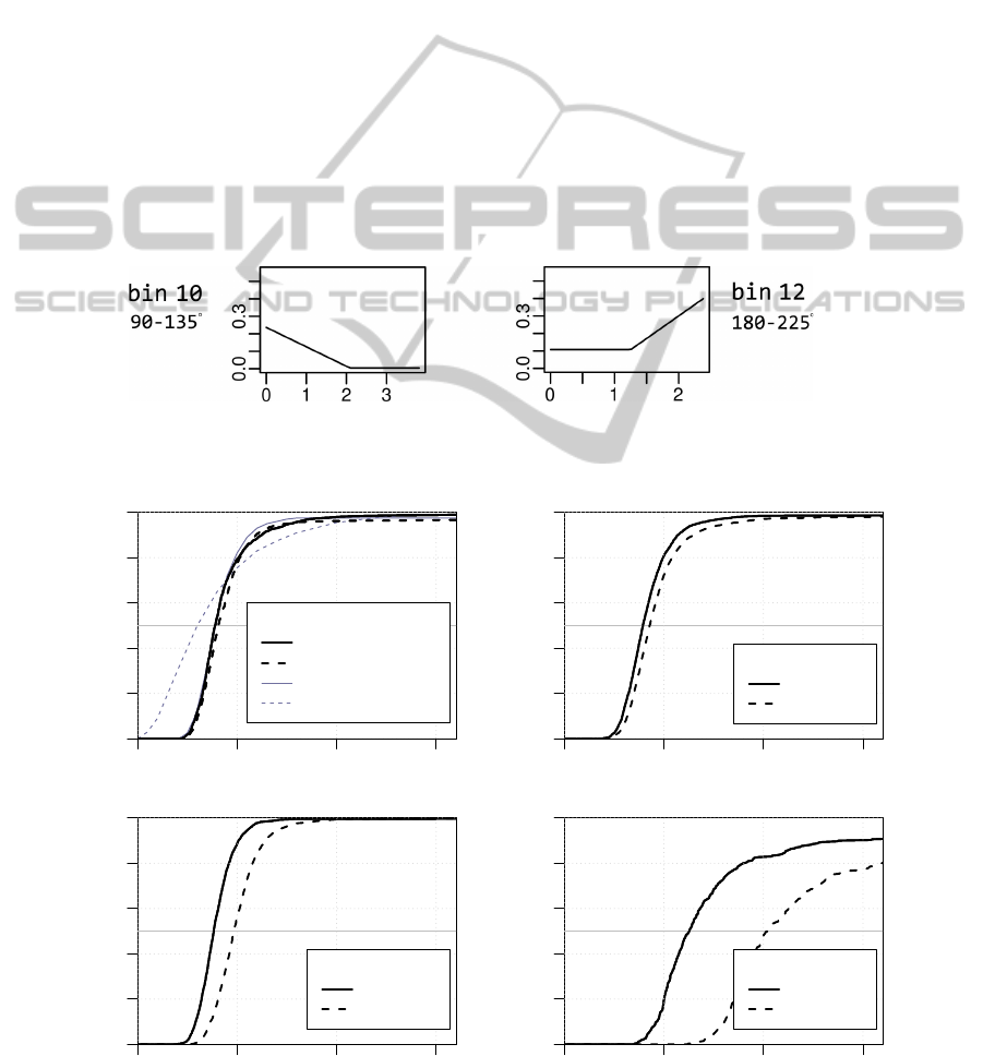
effect of two of the bins is shown in Figure 5. The

same bin can appear in multiple terms, allowing com-

plex non-monotonic regression surfaces (but always

piecewise linear).

MARS has included only certain histogram bins

in the formula (there are 160 bins but only 17 terms

in our example). HAT descriptors lend themselves to

this kind of variable selection. The innate structure

of the image feature makes some bins more important

than others. Furthermore, the trilinear interpolation

Figure 5: The effect of bins 10 and 12 in terms (3) and (4) in the MARS formula above (with the other bins ﬁxed at their

median values). The estimated quality of match is increased by low values in bin 10 and/or high values in bin 12. From

Figure 4, high values in bin 12 are uncommon. Low values are common but uninformative.

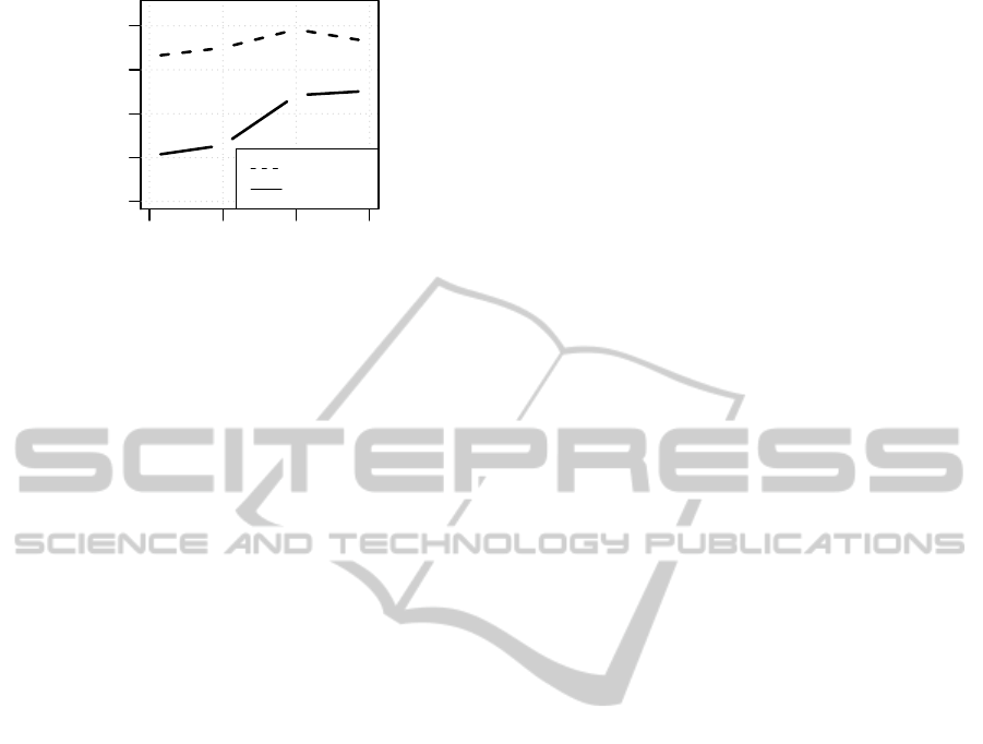
0.00 0.05 0.10 0.15

0.0 0.2 0.4 0.6 0.8 1.0

me17

proportion

BioID

HatAsm

Stasm 3.1

Cootes et al. 2012

Belhuemer et al.

0.00 0.05 0.10 0.15

0.0 0.2 0.4 0.6 0.8 1.0

me17

proportion

XM2VTS

HatAsm

Stasm 3.1

0.00 0.05 0.10 0.15

0.0 0.2 0.4 0.6 0.8 1.0

me17

proportion

PUT

HatAsm

Stasm 3.1

0.00 0.05 0.10 0.15

0.0 0.2 0.4 0.6 0.8 1.0

me17

proportion

Helen

HatAsm

Stasm 3.1

Figure 6: me17 distributions comparing our HatAsm to Stasm Version 3.1.

VISAPP2014-InternationalConferenceonComputerVisionTheoryandApplications

384

●

0 50 100 200

search time in ms

●

Stasm 3.1

HatAsm

BioID 55

XM2VTS 101

PUT 280

Helen 280

Figure 7: Search times (excluding face detection). The

databases are arranged in order of mean inter-pupil dis-

tance (shown after the database name on the horizontal

axis). Times were measured on a 3.4 GHz i7 with the same

datasets as Figure 6. Our software allows 64 bit executables

and use of OpenMP, but for impartial comparison we used

32 bit Microsoft VC10 builds without OpenMP for testing

both implementations.

induces collinearities between nearby bins. When

matching, it may therefore make little difference if we

use a bin or its neighbor. The MARS model building

algorithm will arbitrarily (depending on noise) pick

one or the other. Once the bin is in the formula, the

other bin can be ignored as it brings little new infor-

mation. Usually the ﬁnal formula is so short that eval-

uating it is quicker than it would be to say take the

Euclidean distance between two descriptors. Exploit-

ing structure in the data saves unnecessary calculation

and reduces noise from uninformative variables.

Further details on MARS can be found in (Fried-

man, 1991) and perhaps more accessibly in (Hastie

et al., 2009). We compiled the MARS formulas as

C++ code directly into our application. We performed

MARS model selection (i.e. optimization of the num-

ber of terms) not by using the standard MARS Gen-

eralized Cross Validation but by optimizing descrip-

tor match performance on a tuning set. With smaller

training sets (less than a thousand faces) our experi-

ence has been that linear models can perform as well

as MARS. MARS also allows interactions between

variables, but interactions do not appear to give better

ﬁts in this setting unless large data sets are used (ten

thousand faces).

7 EXPERIMENTS

To summarize, our model differs from the classical

ASM simply in that it incorporates HAT descriptors

and uses MARS to measure descriptor matches. In

this section we refer to this model as a “HatAsm”

model.

We compare the model primarily to the open

source Stasm landmarker (Milborrow and Nicolls,

2008). (Stasm outperformed other public landmark-

ers in three of the four tests in a comprehensive 2013

study (C¸ eliktutan et al., 2013). Stasm uses a combina-

tion of 1D and square gradient descriptors with Ma-

halanobis distances.) We used the version of Stasm

current at the time of writing (Version 3.1), which was

trained on the MUCT data (Milborrow et al., 2010).

For these tests we trained our ASM on the same data

(using the training regimen described at the end of

Section 5). We also used the same OpenCV frontal

face detector (Lienhart and Maydt, 2002) as Stasm

to ﬁnd the face and for initialization the ASM start

shape. After preliminary experimentation on inde-

pendent data, for the tests here our model uses 1D

gradient descriptors at the coarsest pyramid level and

on the jaw points at all pyramid levels, and HAT de-

scriptors otherwise.

We present results in terms of the me17 mea-

sure (Cristinacce and Cootes, 2006), which is the

mean distance between 17 internal face points (Fig-

ure 1) located by the search and the corresponding

manually landmarked points, divided by the distance

between the manual eye pupils. Depending on the ap-

plication, other ﬁtness measures may be more appro-

priate, but the me17 is widely used and forms a con-

venient baseline. Tests using other distance measures

gave results similar to those shown here.

Figure 6 shows results on four different datasets

disjoint from the training data. (As is common prac-

tive, we show results as the cumulative distribution

of ﬁts. The quicker an S curve starts and the faster

it reaches the top, the better the model.) Our imple-

mentation outperforms Stasm 3.1 on all sets except

arguably on the BioID data.

The BioID graph also shows the results of (Bel-

humeur et al., 2011). Apart from the poor perfor-

mance above the 75th percentile, the Belhumeur et al.

results are to our knowledge the best published re-

sults on this set (excluding papers which report re-

sults on subsets or re-marked versions of the BioID

data). However, their landmarker takes on the order

of a second per landmark, whereas ours processes the

entire face in about 50ms. We also show the results

of (Cootes et al., 2012), who estimate the position of

a point by combining the positions estimated by Ran-

dom Forest regressions on nearby patches. The im-

proved results near the top of their curve are perhaps

due to their use of a commercial face detector which

almost certainly outperforms the OpenCV detector.

Both our HatAsm and Stasm are limited to near-

ActiveShapeModelswithSIFTDescriptorsandMARS

385

frontal views by their reliance on a frontal face detec-

tor, so are inappropriate for the Helen set (Le et al.,

2012) with its wide range of poses, but our imple-

mentation fares signiﬁcantly better.

Figure 7 compares search times. Our implemen-

tation is faster than Stasm. The (Cootes et al., 2012)

Random Forest technique (not shown in Figure 7) is

faster than ours, but they ﬁt only 17 points (we ﬁt 76).

Details. The HatAsm and Stasm 3.1 curves in-

clude all faces in the BioID (Jesorsky et al., 2001),

XM2VTS (Messer et al., 1999), and PUT (Kasinski

et al., 2008) sets, and the designated test of the Helen

set (Le et al., 2012). Faces not found by the face de-

tectors are included in these curves, with an me17 of

inﬁnity. For the PUT set several extra points needed

for calculating me17s were manually added before

testing began. For the Helen set we approximated the

pupil and nose points needed for me17s from neigh-

boring points, introducing noise to the results (but

equally for both implementations). The Belhumeur et

al. and Cootes et al. curves were transcribed from ﬁg-

ures in their papers. All other curves were created by

running software on a local machine.

Publication Note. Techniques in this paper have

now been integrated into Stasm to form Stasm Ver-

sion 4.0. Documented source code is available at

www.milbo.users.sonic.net/stasm.

8 DISCUSSION AND FUTURE

DIRECTIONS

We have shown that HAT descriptors together with

MARS work well with ASMs. HAT descriptors out-

perform gradient based descriptors. HAT descriptors

with MARS bring signiﬁcant computational advan-

tages over SIFT descriptors with Mahalanobis dis-

tances or SVMs.

An obvious next step would be to investigate other

modern descriptors such as GLOH (Mikolajczyk and

Schmid, 2005), SURF (Bay et al., 2006), or HOG

(Dalal and Triggs, 2005) descriptors (our HAT de-

scriptors are the same as one variant of HOGs, R-

HOGs). Evidence from other domains indicate that

such alternatives per se may not give ﬁt improvements

over HATs.

In (Milborrow et al., 2013) we extend the model

to non-frontal faces.

In recent years researchers have paid considerable

attention to improving the way the template and shape

models work together. Instead of the rigid separation

between template matching and the shape model of

the classical ASM, one can build a combined model

that jointly optimizes the template matchers and shape

constraints. An early example is the Constrained Lo-

cal Model of (Cristinacce and Cootes, 2006). An

informative taxonomy is given in (Saragih et al.,

2010). Such an approach would probably improve

HAT based landmarkers. The advantages of HATs

are diminished by the classical ASM shape model (the

improvement of HATS over square gradient descrip-

tors is signiﬁcantly larger before the shape constraints

are applied). The match response surfaces over the

search regions are smoother for HATs than for square

gradient descriptors, and this might ease the difﬁcult

optimization task.

REFERENCES

Bay, H., Tuytelaars, T., and Gool, L. V. (2006). SURF:

Speeded Up Robust Features. ECCV.

Belhumeur, P. N., Jacobs, D. W., Kriegman, D. J., and Ku-

mar, N. (2011). Localizing Parts of Faces Using a

Consensus of Exemplars. CVPR.

Belongie, S., Malik, J., and Puzicha., J. (2002). Shape

Matching and Object Recognition Using Shape Con-

texts. PAMI.

Breiman, L. (2001). Random Forests. Machine Learning.

Breiman, L., Friedman, J. H., Olshen, R. A., and Stone,

C. J. (1984). Classiﬁcation and Regression Trees.

Wadsworth.

Castrill

on Santana, M., D

eniz Su

arez, O.,

Hern

andez Tejera, M., and Guerra Artal, C. (2007).

ENCARA2: Real-time Detection of Multiple Faces at

Different Resolutions in Video Streams. Journal of

Visual Communication and Image Representation.

C¸ eliktutan, O., Ulukaya, S., and Sankur, B. (2013). A

Comparative Study of Face Landmarking Techniques.

EURASIP Journal on Image and Video Processing.

http://jivp.eurasipjournals.com/content/2013/1/13/

abstract. This study used Stasm Version 3.1.

Cootes, T., Ionita, M., Lindner, C., and Sauer, P. (2012). Ro-

bust and Accurate Shape Model Fitting using Random

Forest Regression Voting. ECCV.

Cootes, T. F. and Taylor, C. J. (1993). Active Shape Model

Search using Local Grey-Level Models: A Quantita-

tive Evaluation. BMVC.

Cootes, T. F. and Taylor, C. J. (2004). Technical Re-

port: Statistical Models of Appearance for Computer

Vision. The University of Manchester School of

Medicine. http://www.isbe.man.ac.uk/∼bim/Models/

app

models.pdf.

Cootes, T. F., Taylor, C. J., Cooper, D. H., and Graham, J.

(1995). Active Shape Models — their Training and

Application. CVIU.

Cristinacce, D. and Cootes, T. (2006). Feature De-

tection and Tracking with Constrained Local Mod-

els. BMVC. mimban.smb.man.ac.uk/publications/

index.php.

VISAPP2014-InternationalConferenceonComputerVisionTheoryandApplications

386

Dalal, N. and Triggs, B. (2005). Histograms of Oriented

Gradients for Human Detection. CVPR.

Freeman, W. T. and Roth, M. (1995). Orientation His-

tograms for Hand Gesture Recognition. AFGR.

Friedman, J. H. (1991). Multivariate Adaptive Regres-

sion Splines (with discussion). Annals of Statistics.

http://www.salfordsystems.com/doc/MARS.pdf.

Hastie, T., Tibshirani, R., and Friedman, J. (2009). The Ele-

ments of Statistical Learning: Data Mining, Inference,

and Prediction (Second Edition). Springer.

Jesorsky, O., Kirchberg, K., and Frischholz, R. (2001). Ro-

bust Face Detection using the Hausdorff Distance.

AVBPA.

Kanaujia, A. and Metaxas, D. N. (2007). Large Scale

Learning of Active Shape Models. ICIP.

Kasinski, A., Florek, A., and Schmidt, A. (2008). The PUT

Face Database. IPC.

Le, V., Brandt, J., Lin, Z., Boudev, L., and Huang,

T. S. (2012). Interactive Facial Feature Localization.

ECCV. http://www.ifp.illinois.edu/ vuongle2/helen.

Leathwick, J., Rowe, D., Richardson, J., Elith, J., and

Hastie, T. (2005). Using Multivariate Adaptive Re-

gression Splines to Predict the Distributions of New

Zealand’s Freshwater Diadromous Fish. Freshwa-

ter Biology, 50, 2034-2052. http://www.botany.

unimelb.edu.au/envisci/about/staff/elith.html.

Li, Z., Imai, J.-i., and Kaneko, M. (2009). Facial Feature

Localization using Statistical Models and SIFT De-

scriptors. Robot and Human Interactive Communica-

tion.

Lienhart, R. and Maydt, J. (2002). An Extended Set of Haar-

Like Features for Rapid Object Detection. IEEE ICP.

Lowe, D. G. (2004). Distinctive Image Features from Scale-

Invariant Keypoints. IJCV.

Messer, K., Matas, J., Kittler, J., Luettin, J., and Maitre, G.

(1999). XM2VTS: The Extended M2VTS Database.

AVBPA.

Mikolajczyk, K. and Schmid, C. (2005). A Performance

Evaluation of Local Descriptors. PAMI.

Milborrow, S., Bishop, T. E., and Nicolls, F. (2013). Mul-

tiview Active Shape Models with SIFT Descriptors for

the 300-W Face Landmark Challenge. ICCV.

Milborrow, S., Morkel, J., and Nicolls, F. (2010).

The MUCT Landmarked Face Database. Pat-

tern Recognition Association of South Africa.

http://www.milbo.org/muct.

Milborrow, S. and Nicolls, F. (2008). Locating Facial Fea-

tures with an Extended Active Shape Model. ECCV.

Querini, M. and Italiano, G. F. (2012). Facial Biometrics

for 2D Barcodes. Computer Science and Information

Systems.

Rattani, A., Kisku, D. R., Lagorio, A., and Tistarelli, M.

(2007). Facial Template Synthesis based on SIFT Fea-

tures. Automatic Identiﬁcation Advanced Technolo-

gies.

Saragih, J., Lucey, S., and Cohn, J. (2010). Deformable

Model Fitting by Regularized Landmark Mean-Shifts.

IHCV.

Shi, Y. and Shen, D. (2008). Hierarchical Shape Statisti-

cal Model for Segmentation of Lung Fields in Chest

Radiographs. MICCAI.

Vogel, C., de Sousa Abreu, R., Ko, D., Le, S., Shapiro,

B. A., Burns, S. C., Sandhu, D., Boutz, D. R., Mar-

cotte, E. M., and Penalva, L. O. (2010). Sequence

signatures and mRNA concentration can explain two-

thirds of protein abundance variation in a human cell

line. Molecular Systems Biology.

Zhang, J. and Chen, S. Y. (2008). Combination of Local

Invariants with an Active Shape Model. BMEI.

Zhang, L., Tjondronegoro, D., and Chandran, V. (2011).

Geometry vs. Appearance for Discriminating between

Posed and Spontaneous Emotions. NIP.

Zhou, D., Petrovska-Delacr

etaz, D., and Dorizzi, B. (2009).

Automatic Landmark Location with a Combined Ac-

tive Shape Model. BTAS.

ActiveShapeModelswithSIFTDescriptorsandMARS

387