
A Saliency-based Framework for 2D-3D Registration
Mark Brown, Jean-Yves Guillemaut and David Windridge
Centre for Vision, Speech and Signal Processing, University of Surrey, Guildford, U.K.
Keywords:
Pose Estimation, Registration, Saliency.
Abstract:
Here we propose a saliency-based filtering approach to the problem of registering an untextured 3D object to a
single monocular image. The principle of saliency can be applied to a range of modalities and domains to find
intrinsically descriptive entities from amongst detected entities, making it a rigorous approach to multi-modal
registration. We build on the Kadir-Brady saliency framework due to its principled information-theoretic
approach which enables us to naturally extend it to the 3D domain. The salient points from each domain are
initially aligned using the SoftPosit algorithm. This is subsequently refined by aligning the silhouette with
contours extracted from the image. Whereas other point based registration algorithms focus on corners or
straight lines, our saliency-based approach is more general as it is more widely applicable e.g. to curved
surfaces where a corner detector would fail. We compare our salient point detector to the Harris corner and
SIFT keypoint detectors and show it generally achieves superior registration accuracy.
1 INTRODUCTION
The increase in available 3D data over the last decade
has naturally led to the problem of its registration
with 2D images. It has applications in object recog-
nition, robotics and medical imaging, where in par-
ticular real-time solutions are required (van de Kraats
et al., 2004; Gendrin et al., 2011).
While there is a significant amount of 3D data that
contains texture information, for example acquired
from Structure from Motion or multi-viewreconstruc-
tion techniques, here we consider the problem where
the data is untextured; often obtained from LiDAR or
other forms of laser scanner. This constraint makes
it significantly more challenging, if the 3D data were
textured, point correspondences could be initialised
by, for example, using the SIFT descriptor from View-
point Invariant Patches (Wu et al., 2008). However,
for untextured 3D data these descriptors are inappli-
cable since there is no longer a common modality to
be described.
The 2D / 3D registration problem can be seen as
an instantiation of the more general multi-modal reg-
istration problem, an area that has received signifi-
cant attention in computer vision (van de Kraats et al.,
2004; Gendrin et al., 2011; Mastin et al., 2009; Eg-
nal, 2000). While there exist a number of methods
that can perform this with a good initial alignment,
e.g. 2D / 3D registration in medical imaging using
fiducial markers (van de Kraats et al., 2004) or cross-
spectral stereo matching (Egnal, 2000), the less con-
strained case without these priors remains largely un-
solved. This is because the methods relying on a good
initial alignment often use computationally expensive
measures such as Mutual Information (Egnal, 2000)
and so are infeasible when considering all possible
alignments.
The main contribution of this paper is its advoca-
tion of saliency-based filtering for the 2D / 3D regis-
tration problem. Saliency is a broad term that refers to
the idea that certain parts of an image are more infor-
mative or distinctive than other areas and these parts
represent the intrinsic and underlying aspects of the
object. As such, it is not domain or modality specific,
making it a very general approach to multi-modal reg-
istration. Further, it is seen as an approximation to
the Human Visual System (HVS) which is capable
of solving a variety of vision and registration tasks
very efficiently. The structure of saliency detectors
can be varied since the definition is broadly specified;
the aim is often to extract features that have a high re-
peatability with respect to keypoints people have la-
beled as salient (Judd et al., 2012). As such, the two
detectors the saliency detector is compared to - the
Harris Corner detector and SIFT - could arguably both
be considered saliency detectors in certain contexts.
While there are a range of saliency detectors to
choose from (Itti, 2000; Kadir and Brady, 2001; Judd
265
Brown M., Guillemaut J. and Windridge D..
A Saliency-based Framework for 2D-3D Registration.
DOI: 10.5220/0004675402650273
In Proceedings of the 9th International Conference on Computer Vision Theory and Applications (VISAPP-2014), pages 265-273
ISBN: 978-989-758-003-1
Copyright
c
2014 SCITEPRESS (Science and Technology Publications, Lda.)

et al., 2012; Lee et al., 2005), we use the Kadir-Brady
detector due to its principled information-theoretic
approach. We generalise it over an arbitrary number
of dimensions and implement a curvature based ex-
tension to the 3D domain. It extracts salient points
by maximising the Shannon entropy in scale-space;
a measure that has been used in 2D / 3D and cross-
spectral registration before in the form of Mutual In-
formation (MI) (Mastin et al., 2009; Egnal, 2000)
however MI is too costly in our case as we do not
assume a good initial alignment.
After extracting salient points from both domains,
we seek to align them. However, as descriptors are
typically inapplicable in multi-modal data no corre-
spondences can be initialised; hence the ‘Simultane-
ous Pose and Correspondence’ (SPC) problem has to
be solved. For this we use the SoftPosit algorithm
(David et al., 2002) to initially align the data and the
registration is refined by aligning the edges of the sil-
houette with edges from the image. Whereas other
methods e.g. (Mastin et al., 2009) put a strong prior
on the initial alignment, the SoftPosit point based
method is able to consider a large variety of align-
ments (all rotations and limited translations) within a
reasonable amount of time (5 minutes on a standard
single core CPU).
The structure of this paper is as follows: In Sec-
tion 2, we give an outline of related work in 2D / 3D
registration. In Section 3 we present our methodol-
ogy; in Section 4 our experiments and conclusions are
presented in Section 5.
2 RELATED WORK
2D / 3D registration has received a significant amount
of attention, particularly in the medical domain,
where multi-modal (e.g. CT, MRI, 3D Rotational
X-ray (van de Kraats et al., 2004)) registration is of
great importance. (van de Kraats et al., 2004) evalu-
ate a number of algorithms for this and classify them
as intensity-based, gradient-based, feature-based or
hybrid-based. Algorithms outside of the medical
imaging domain are usually feature-, intensity-, or
learning-based. Registration in medical imaging typ-
ically involves using fiducial markers for an initial
alignment and so the problem becomes one of refine-
ment.
Intensity based methods typically project the 3D
data and use correlation measures such as mutual
information or cross-correlation to refine the regis-
tration (Kotsas and Dodd, 2011). These techniques
have been used in cross-spectral stereo matching (Eg-
nal, 2000) where the offset that maximises the mu-
tual information or correlation is determined to be
the correct offset. It has also been used by (Mastin
et al., 2009) where the authors match a LiDAR scan
to an image using Mutual Information. However, the
authors acknowledge the sensitivity to initialisation,
saying that they do not initialise the yaw or pitch to
more than 0.5 degrees from the ground truth in their
experiments. It would be computationally infeasible
when sampling without these priors.
Feature based methods extract features such as
points or lines, and match these up, often without as-
suming any knowledge about their correspondences
(hence solving for the pose and the correspondences).
A number of papers have attempted to solve the Si-
multaneous Pose and Correspondence (SPC) problem
from these points, a problem also addressed in 3D-
3D registration. With a good enough initial align-
ment, matching can be achieved through Iterative
Closest Point (ICP). This can be made more robust
through Expectation-Maximisation ICP (Granger and
Pennec, 2002) or Levenberg-Marquardt ICP (Fitzgib-
bon, 2001) who further describes the use of differ-
ent kernels to deal with outliers and shows their pro-
posed method increasing the basin of convergence
over other variants of ICP. A well known solution to
SPC, and the one used here, is the SoftPosit algorithm
(David et al., 2002). Unlike ICP, this allows weighted
correspondences between points rather than the bi-
nary assignment in ICP, allowing it to better avoid lo-
cal maxima during convergence. It will be discussed
further in Section 3.3.
More recently (Moreno-Noguer et al., 2008)
solved the SPC problem by modeling initialisations
as a Gaussian Mixture Model and using each com-
ponent to initialise a Kalman filter. They also intro-
duced priors on the camera pose; for example the
camera is always above the ground and pointing to-
wards the object. It performs just as well as SoftPosit
in a similar amount of time except in large amounts of
clutter, where SoftPosit is outperformed by it. Also,
(Enqvist et al., 2009) solved the SPC problem by de-
termining which pairs of correspondences are infea-
sible and sought to maximise the number of corre-
spondences that are feasible. This is done using an
heuristic branch and bound technique and the authors
achieve results comparable to state of the art.
Machine learning algorithms are evident in the lit-
erature for the 2D / 3D registration problem, specifi-
cally in face recognition. In general, the main draw-
back with this approach is the time spent in label-
ing and learning the model. (Yang et al., 2008)
use Canonical Correlation Analysis (CCA) for face
recognition to learn a correlation between image fea-
tures and 3D features of face data. In this applica-
VISAPP2014-InternationalConferenceonComputerVisionTheoryandApplications
266
tion, an image and a 3D mesh of a face are compared:
if there is sufficient correlation then it is deemed a
match.
2.1 Saliency-based Methods
We use Kadir-Brady saliency (Kadir and Brady, 2001;
?) due to its applicability in different modalities re-
sulting from a principled information-theoretic ap-
proach. Other forms of saliency are not so easy to
extend to 3D e.g. Itti-Koch saliency (Itti, 2000) relies
on colour and centre-surround operations that aim to
replicate how the human visual system works. (Lee
et al., 2005) determine the saliency of a 3D mesh
through weighting curvatures in scale space to return
a saliency value for each point; this is not as general
as Kadir-Brady which only requires a histogram.
Saliency has already been applied in the 2D / 3D
registration problem in medical imaging by (Chung
et al., 2004). Here, the authors learn a saliency map
through eye-tracking of volunteers. By focusing on
registering only on the region of the image that is
salient, the authors increase the accuracyof the results
whilst reducing the computation time. This is differ-
ent from what is proposed here because (Chung et al.,
2004) uses a ground truth saliency map constructed
through using eye tracking software; no salient algo-
rithm was used. Instead, we propose a framework for
2D / 3D registration that can be applied to the general
multi-modal registration problem.
3 METHODOLOGY
We wish to register a 3D model to an image. To do so,
N
I
salient image points {x
i
}
N
I
i=1
and N
W
salient mesh
points { X
j
}
N
W
j=1
are extracted in the first stage of the
methodology. This is achieved using the generalised
Kadir-Brady saliency detector in each modality (see
Sections 3.1 and 3.2).
The second stage of the methodology aims to de-
termine the transformation that matches these points.
This requires the SPC problem to be solved since no
putative matches may be found, for which SoftPosit
(David et al., 2002) is used.
However, this is only possible if the two sets of
salient points have a sufficiently high repeatability.
This may not be the case: in particular the image
points may exhibit projective saliency, whereby they
are salient because they lie on the edge of the pro-
jected model, due to the viewing angle (i.e. transfor-
mation between modalities) rather than the model’s
intrinsic properties. An example of this is given in
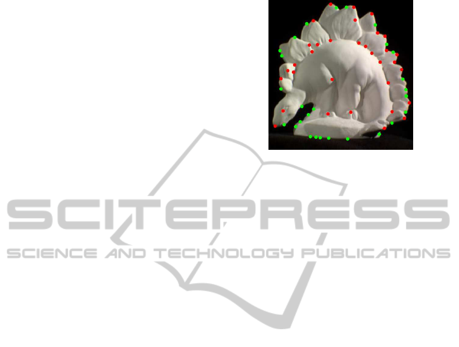
Figure 1: An illustration of different types of saliency. The
red points are salient due to the intrinsic properties of the
model whereas the green points exhibit projective saliency.
Figure 1. Projective saliency is accounted for by ex-
tracting points on the edge of the silhouette (S) of the
mesh and measuring their alignment with {x
i
}
N
I
i=1
- a
detailed explanation is given in Section 3.3.
The final stage of the methodology takes the
best scoring 1% of transformations from the previ-
ous stage and refines them by further matching edges
from 2D (extracted using the Canny edge detector)
with the boundary of the 3D silhouette - a detailed
explanation of this is given in Section 3.4. A diagram
showing the pipeline of the methodology is given in
Figure 2.
3.1 The Generalised Kadir-Brady
Saliency Detector
The Kadir-Brady detector is here abstracted to R
n
.
This is constructed using a set of points {x
i
∈ R
n
},
a set of scales {s
1
,...,s
K
} and a histogram with val-
ues
v
1,x,s
k
,...,v
R,x,s
k
associated with a point x over
a given scale s
k
. The Kadir-Brady detector uses this
histogram about each point for each scale and de-
termines where the histogram’s entropy is peaked in
scale space. The higher this peak is above its neigh-
bour’s scales, the higher the saliency of that point is
defined to be.
More formally, for a point x, a scale s
k
, and a his-
togram with values
v
1,x,s
k
,...,v
R,x,s
k
, the entropy of
x is defined as:
H
x,s
k
= −
R
∑
i=1
P(v
i,x,s
k
)log
2
(P(v
i,x,s
k
)) (1)
where P(v
i,x,s
k
) is the probability of the histogram
taking the value v
i
at scale s
k
from x. This is
taken from a frequentist approach, i.e. P(v
i,x,s
k
) =
v
i,x,s
k
/
R
∑
j=1
v
j,x,s
k
. (Shao et al., 2007) make this step
ASaliency-basedFrameworkfor2D-3DRegistration
267
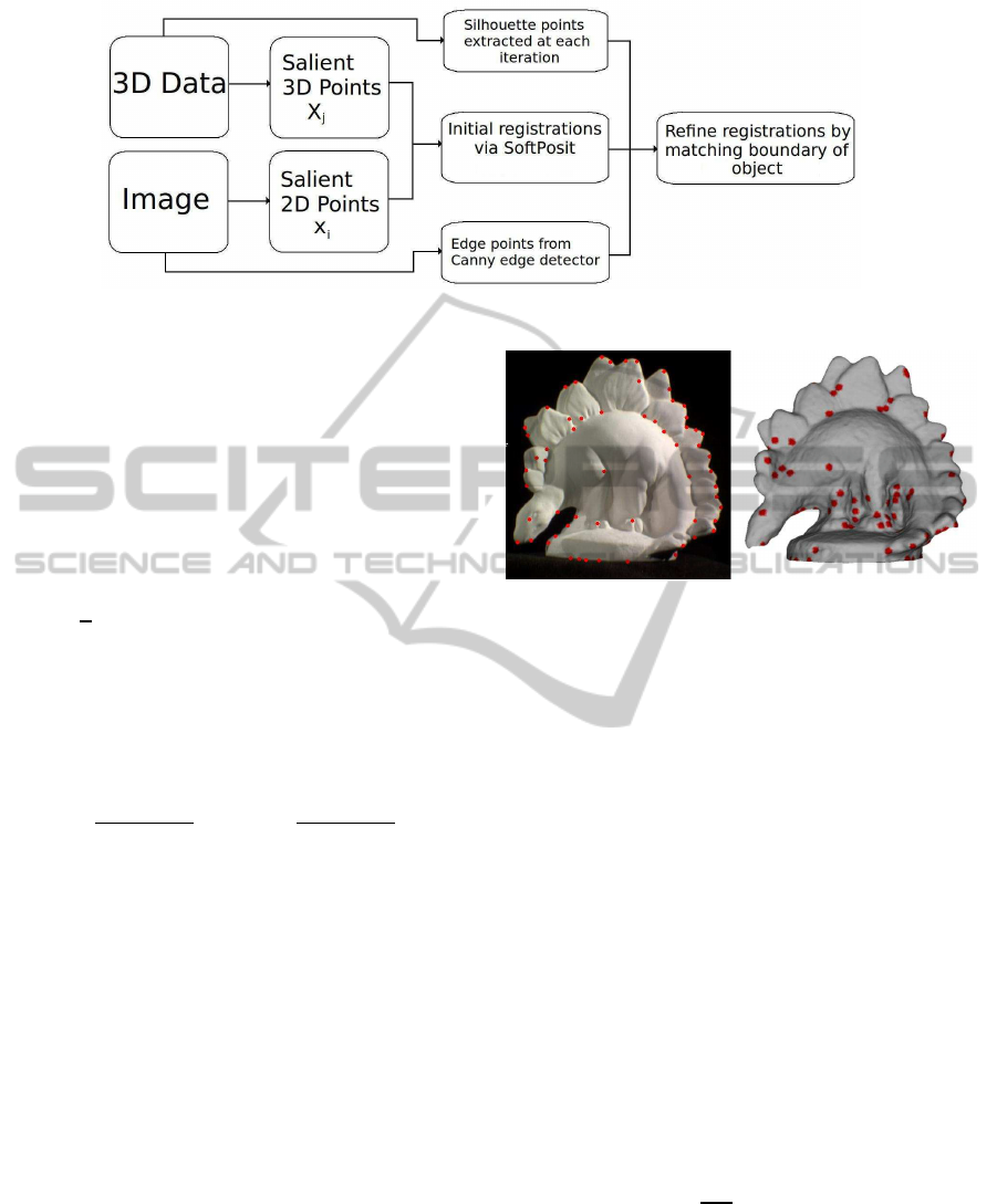
Figure 2: Pipeline of methodology for 2D / 3D registration.
more robust by weighting points by twice as much if
they are within s
k−1
of x. This is used here as the au-
thors demonstrate an increase in the repeatability by
10% compared to no weighting.
After computing the entropy of each point at each
scale (as above) only the scale-space points for which
the entropy is peaked above its neighbouring two
scales are retained. This is then weighted by how dis-
similar the PDF is from these two scales:
W
x,s
k
=
1
2
C
1
R
∑
i=1
P(v
i,x,s
k+1
) −P(v
i,x,s
k
)
+
C
2
R
∑
i=1
P(v
i,x,s
k
) −P(v
i,x,s
k−1
)
(2)
where C
1
and C
2
are constants that make the compar-
ison scale invariant:
C
1
=
N
s
k+1
N
s
k+1
−N
s
k
C
2
=
N
s
k
N
s
k
−N
s
k−1
(3)
and where N
s
k
is the number of points within s
k
of x,
i.e. N
s
k
=
R
∑
i=1
v
i,x,s
k
. The final saliency measure Y
x,s
k
is
then the product of the two measures H
x,s
k
and W
x,s
k
.
These salient points are subsequently clustered
into circular salient regions using an heuristic cluster-
ing algorithm according to (Kadir and Brady, 2001).
Its purpose is to make it more robust to noise as this
would otherwise act as a randomiser and increase the
entropy. The centre of each circular region is defined
to be the salient point returned by the detector,and has
an associated scale and saliency value. An example
of points extracted from the generalised Kadir-Brady
saliency detector is given in Figure 3.
The original Kadir-Brady detector for images (R
2
)
constructs a 256-bin histogram of pixel intensities
about each pixel taken from a circular neighbourhood
of radius s
k
. The radius ranges from three pixels to 21
in intervals of three.
Figure 3: Detected points of the Middlebury dinosaur using
the standard 2D Kadir-Brady detector (left) and its exten-
sion to 3D mesh-based data (right).
3.2 The 3D Kadir-Brady Saliency
Detector
While the scale-space concept is the same in 3D, the
descriptor histogram to use is less obvious. After
some experiments, we adopt a curvature-based detec-
tor, the same as in (Lee et al., 2005). For this the
mean curvature (the average of the two principal cur-
vatures) is used, where the principal curvatures at x
are defined to be the eigenvalues of the shape operator
at x, and are calculated using the algorithm presented
by (Taubin, 1995). Since this algorithm can produce
abnormally large curvatures for some points due to
floating point errors, in our algorithm those with the
top 0.5% of all curvature values have their curvature
value capped. Denoting the maximum curvature by
M, a 30-bin histogram around point x with scale s
k
is constructed as follows: For each point x
j
that is
within s
k
of x denote its curvature as x
c
j
. Then insert
this into bin number ⌊
30x
c
j
M
⌋, i.e. construct bins of uni-
form width ranging from curvatures 0 to M. Thus the
value of each bin in the histogram can be expressed
as:
VISAPP2014-InternationalConferenceonComputerVisionTheoryandApplications
268

v
i,x,s
k
=
∑
x
j
:|x−x
j
|<s
k
δ(⌊
30x
c
j
M
⌋,i)
+
∑
x
j
:|x−x
j
|<s
k−1
δ(⌊
30x
c
j
M
⌋,i) (4)
where ⌊x⌋ denotes the greatest integer smaller than x
and δ the Kronecker delta function.
Seven scales are used as in the 2D case. Here the
lowest scale is 0.3% of the length of the diagonal of
the bounding box of the model, and this increases in
0.3% intervals up to 2.1%.
3.3 The SoftPosit Algorithm
The SoftPosit algorithm (David et al., 2002) attempts
to solve the SPC Problem: for image points {x
i
}
N
I
i=1
and model points {X
j
}
N
W
j=1
it aims to find:
argmin
R,T,P
N
I
∑
i=1
N
W
∑
j=1
P
i, j
||K(RX
j
+ T) −x
i
||
2
(5)
where K is the known camera intrinsics, R ∈ SO(3),
T is a 3x3 translation vector and P is a permutation
matrix whose entries are P
i, j
= 1 if x
i
matches X
j
and
0 otherwise. A brief outline of the SoftPosit algorithm
is given here, with more detail in (David et al., 2002).
The SoftPosit algorithm iteratively switches be-
tween assigning correspondences (P) (involving mul-
tiple, weighted correspondences from each point) and
solving the pose (R and T) from these weighted corre-
spondences. Furthermore, the parameter that controls
this weighting (β) can be seen as a simulated anneal-
ing parameter, meaning the correspondences tend to-
wards the binary ‘one correspondence per point’ as
required in Equation 5. For comparison with Section
3.4, the update step is as follows:
Inputs: N
W
world points, N
I
image points, hypothe-
sised pose.
Outputs: Updated pose.
1. For each world / image coordinate pair (X
j
, x
i
),
project x
i
to the same depth as X
j
using a per-
spective projection, then project this back onto the
image plane under a Scaled Orthographic Projec-
tion (SOP) - call this p
i
. Define the projection of
X
j
under a SOP as q
j
. Let d
i, j
= |p
i
−q
j
|.
2. Compute a matrix of weights m
i, j
=
γexp(−β(d
i, j
− α)) for β = 0.004, α = 1,
γ = 1/(max{N
W
,N
I
} + 1). Also ∀ i, j set
m
i,N
W
+1
= m
N
I
+1, j
= γ : this represents the
probability of a point having no correspondence.
3. Use Sinkhorn’s method to normalise each row and
column (apart from the last ones) of this matrix.
This is achieved by alternately normalising each
row and column.
4. Use m
i, j
as the weights for weighted corre-
spondences to update the pose by minimising a
weighted sum (specifically Equation 5 with P
i, j
=
m
i, j
). This is achieved simply by setting the
derivative of the objective function to zero.
The algorithm is iterated from the first stage with
β increasing by a factor of 1.05 each iteration - this
has the effect of weighting close points significantly
higher.
What is defined here as projective saliency is now
taken into account by extracting points on the edge
of the silhouette (S) of the model and aligning these
with the image points. Therefore, (5) is altered and
the objective is to find:
argmin
R,T
N
W
∑
j=1
N
I
min
i=1
||K(RX
j
+ T) −x
i
||
2
+
N
I
∑
i=1
min
j∈W
||K(RX
j
+ T) −x
i
||
2
(6)
where W represents the union of the original salient
3D points and the 3D points on the boundary of the
silhouette S (and is thus dependent on R and T). Note
that (6) no longer depends on P; this is because the
problem is no longer symmetric (image points may
lie on the boundary but not vice versa). Obtaining
the silhouette at every iteration is an expensive opera-
tion and is only relevant when the hypothesised pose
is within the vicinity of the solution. Therefore, the
points are initially aligned according to (5) by Soft-
Posit and scored according to (6), which is subse-
quently minimised in Section 3.4.
In the current implementation, 50 iterations are
carried out from 500 random initial poses, for which
random rotation matrices were generated using the
method described in (Arvo, 1992). Further, OpenGL
is used to render the 3D model and points that are not
visible are not included in the update step. As this is
computationally expensive, it is only done when the
pose is sufficiently different from the previous time
the visibility condition was checked. This difference
is measured as the sum over all elements in R and T of
the absolute difference between the two poses. From
these 500 initialisations, the lowest scoring 1% are se-
lected according to (6).
3.4 Boundary Matching
After an initial alignment is obtained, the top 1% are
subsequently refined by matching the boundary of the
ASaliency-basedFrameworkfor2D-3DRegistration
269

silhouette with the outer edges of the image as well
as matching the original 2D and 3D salient points. A
Canny edge detector is first used on the image and
points are extracted on the exterior contour from this.
With these E exterior points, there are now N
W
world
coordinates and (N
I
+ E) image points and (6) is min-
imised with this new set of image points. The update
step is adjusted as follows:
Inputs: N
W
world points, (N
I
+ E) image points, hy-
pothesised pose, 3D mesh.
Outputs: Updated pose.
1. Compute d
i, j
between the N
W
world points and all
(N
I
+ E) image points.
2. For each of the (N
I
+ E) image points, compute
the distance between it and the nearest point that
is on the edge of the silhouette. (Computing the
distance between it and all points on the edge of
the silhouette is too computationally expensive.)
3. Construct the matrix of weights m
i, j
as appropri-
ate, taking into account an image point may be
matched with its nearest point on the silhouette.
This leads to a (N
W
+ 2) × (N
I
+ E + 1) matrix.
Apply Sinkhorn’s method for the same purpose as
in Section 3.3.
4. Use these weighted correspondencesto update the
pose, similar to Section 3.3.
Again, β is increased by a factor of 1.05 at each it-
eration. The score is calculated in the same way as be-
fore, except now it uses all (N
I
+ E) image points in-
stead of the N
I
originally extracted. The lowest scor-
ing match is deemed the correct alignment.
4 EXPERIMENTS
4.1 Experimental Setup
We applied our algorithm to six datasets; two real
and four synthetic. The synthetic datasets are the
Stanford bunny and Stanford dragon, and the horse
and angel from the Large Geometric Models Archive
from Georgia Institute of Technology. For the syn-
thetic datasets, textureless images were generated us-
ing POV-Ray from a random angle (Arvo, 1992) and
fixed translation, using a point light source at the same
location as the camera. The two real datasets are the
dinosaur and temple from Middlebury’s multi-view
reconstruction dataset (Seitz et al., 2006). Since this
does not include the ground truth, we use the 3D
reconstruction provided by (Guillemaut and Hilton,
2011). These images contain texture information of
the model while the 3D data does not, adding an-
other layer of difficulty. An example image from each
dataset is shown on the right of Figure 4. In all cases,
we attempted to align 30 images independently to the
model.
For each attempted registration, we extracted 160
points from the 3D structure and 80 from the image.
We extract these using the generalised Kadir-Brady
saliency method described here, and using the Harris
corner detector and the SIFT keypoint detector, both
of which have a respective implementation in 3D (As
there is no texture in the models, SIFT uses the cur-
vature value instead). All three of these keypoint de-
tectors return a response value which is used to rank
them so as to obtain the optimal keypoints. We then
follow the methodology described in Section 3, ini-
tialising SoftPosit with 500 random poses.
To generate the poses, we assume no prior infor-
mation on the rotation and so we generate random ro-
tation matrices according to (Arvo, 1992). However,
we initialise the translation such that the mean of the
3D data is in the centre of the image (which is the
case in the synthetic data, and is sufficiently close for
the real data) and initialise a random depth within 5%
from the ground truth. Whilst we could have sampled
over a larger range of translations, this is unrealistic
as often an image of a model is focused at a suitable
location to capture all of the structure.
4.2 Results and Discussion
We define three distance measures to compare the
hypothesised registration with its ground truth. The
first measure is a comparison of rotations. There
are a number of ways to compare rotation matrices
(Huynh, 2009). Here, we define the angle between
the rotation R and its ground truth rotation R
gt
as
E
rot
(θ) = arccos(Ru·R
gt
u) with u =
1
√
3
[1,1,1]
T
. Sec-
ondly, we measure the distance between the hypothe-
sised camera centre and the ground truth camera cen-
tre in normalised 3D coordinates (E
dist
). Finally we
introduce the projection error: it is calculated by pro-
jecting the model using the hypothesised projection
and comparing it with the ground truth projection by
comparing the two generated areas A and B. The error
is defined as E
proj
(%) =
(A∪B)\(A∩B)
A∪B
.
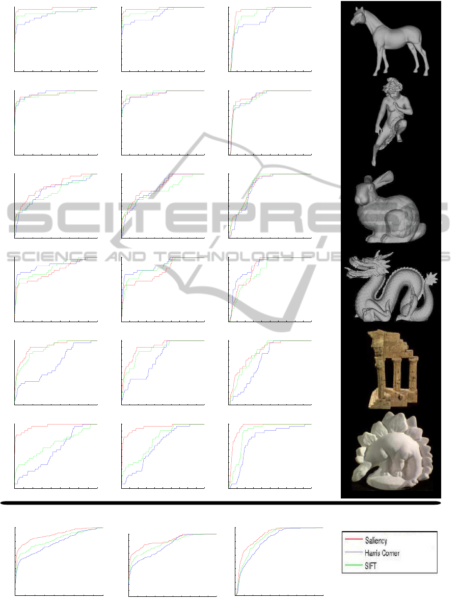
The cumulative frequency curves for these mea-
sures are shown in Figure 4 for individual datasets and
their average across all datasets.
Overall, the saliency detector produced the best
results, particularly on the real data and the horse.
It performed similarly to the other detectors for the
Stanford bunny and the angel. This is shown by
the different areas under the cumulative frequency
VISAPP2014-InternationalConferenceonComputerVisionTheoryandApplications
270
0 20 40 60 80 100 120 140 160 180
0
0.1
0.2
0.3
0.4
0.5
0.6
0.7
0.8
0.9
1
Degrees from ground truth
Cumulative Frequency
Horse
0 20 40 60 80 100 120 140 160 180
0
0.1
0.2
0.3
0.4
0.5
0.6
0.7
0.8
0.9
1
Degrees from ground truth
Cumulative Frequency
Angel
0 20 40 60 80 100 120 140 160 180
0
0.1
0.2
0.3
0.4
0.5
0.6
0.7
0.8
0.9
1
Degrees from ground truth
Cumulative Frequency
Stanford Bunny
0 20 40 60 80 100 120 140 160 180
0
0.1
0.2
0.3
0.4
0.5
0.6
0.7
0.8
0.9
1
Degrees from ground truth
Cumulative Frequency
Stanford Dragon
0 20 40 60 80 100 120 140 160 180
0
0.1
0.2
0.3
0.4
0.5
0.6
0.7
0.8
0.9
1
Degrees from ground truth
Cumulative Frequency
Middlebury Temple
0 20 40 60 80 100 120 140 160 180
0
0.1
0.2
0.3
0.4
0.5
0.6
0.7
0.8
0.9
1
Degrees from ground truth
Cumulative Frequency
Middlebury Dinosaur
0 0.2 0.4 0.6 0.8 1 1.2 1.4 1.6 1.8 2
0
0.1
0.2
0.3
0.4
0.5
0.6
0.7
0.8
0.9
1
Distance from Camera
Cumulative Frequency
Horse
0 0.2 0.4 0.6 0.8 1 1.2 1.4 1.6 1.8 2
0
0.1
0.2
0.3
0.4
0.5
0.6
0.7
0.8
0.9
1
Distance from Camera
Cumulative Frequency
Angel
0 0.2 0.4 0.6 0.8 1 1.2 1.4 1.6 1.8 2
0
0.1
0.2
0.3
0.4
0.5
0.6
0.7
0.8
0.9
1
Distance from Camera
Cumulative Frequency
Stanford Bunny
0 0.2 0.4 0.6 0.8 1 1.2 1.4 1.6 1.8 2
0
0.1
0.2
0.3
0.4
0.5
0.6
0.7
0.8
0.9
1
Distance from Camera
Cumulative Frequency
Stanford Dragon
0 0.2 0.4 0.6 0.8 1 1.2 1.4 1.6 1.8 2
0
0.1
0.2
0.3
0.4
0.5
0.6
0.7
0.8
0.9
1
Distance from Camera
Cumulative Frequency
Middlebury Temple
0 0.2 0.4 0.6 0.8 1 1.2 1.4 1.6 1.8 2
0
0.1
0.2
0.3
0.4
0.5
0.6
0.7
0.8
0.9
1
Distance from Camera
Cumulative Frequency
Middlebury Dinosaur
0 20 40 60 80 100 120 140 160 180
0
0.1
0.2
0.3
0.4
0.5
0.6
0.7
0.8
0.9
1
Degrees from ground truth
Cumulative Frequency
All Datasets
0 0.2 0.4 0.6 0.8 1 1.2 1.4 1.6 1.8 2
0
0.1
0.2
0.3
0.4
0.5
0.6
0.7
0.8
0.9
1
Distance from Camera
Cumulative Frequency
All Datasets
0 0.1 0.2 0.3 0.4 0.5 0.6 0.7 0.8 0.9 1
0
0.1
0.2
0.3
0.4
0.5
0.6
0.7
0.8
0.9
1
Projection Overlap
Cumulative Frequency
Horse
0 0.1 0.2 0.3 0.4 0.5 0.6 0.7 0.8 0.9 1
0
0.1
0.2
0.3
0.4
0.5
0.6
0.7
0.8
0.9
1
Projection Overlap
Cumulative Frequency
Angel
0 0.1 0.2 0.3 0.4 0.5 0.6 0.7 0.8 0.9 1
0
0.1
0.2
0.3
0.4
0.5
0.6
0.7
0.8
0.9
1
Projection Overlap
Cumulative Frequency
Stanford Bunny
0 0.1 0.2 0.3 0.4 0.5 0.6 0.7 0.8 0.9 1
0
0.1
0.2
0.3
0.4
0.5
0.6
0.7
0.8
0.9
1
Projection Overlap
Cumulative Frequency
Stanford Dragon
0 0.1 0.2 0.3 0.4 0.5 0.6 0.7 0.8 0.9 1
0
0.1
0.2
0.3
0.4
0.5
0.6
0.7
0.8
0.9
1
Projection Overlap
Cumulative Frequency
Middlebury Dinosaur
0 0.1 0.2 0.3 0.4 0.5 0.6 0.7 0.8 0.9 1
0
0.1
0.2
0.3
0.4
0.5
0.6
0.7
0.8
0.9
1
Projection Overlap
Cumulative Frequency
Middlebury Temple
0 0.1 0.2 0.3 0.4 0.5 0.6 0.7 0.8 0.9 1
0
0.1
0.2
0.3
0.4
0.5
0.6
0.7
0.8
0.9
1
Projection Overlap
Cumulative Frequency
All Datasets
Figure 4: Images of the datasets and cumulative frequency curves for each error measure. From left to right: Rotation error;
Distance between camera centres; Projective error; image of dataset. From top to bottom: horse; angel; Stanford bunny;
Stanford dragon; Middlebury temple; Middlebury Dinosaur; Average across all datasets.
ASaliency-basedFrameworkfor2D-3DRegistration
271

curve for each point detector when averaged across
all datasets:
Dataset / Error Type E
rot
(θ) E
dist
E
proj
(%)
Harris 140 1.63 0.81
SIFT 149 1.70 0.85
Saliency 169 1.72 0.88
Whilst our method worked well on the Stanford
dragon, it was outperformed by the Harris corner de-
tector and SIFT; this may be due to the large amount
of small corners on it, allowing the other methods to
be better suited. In particular, Kadir-Brady saliency
may not work as well for small features since their en-
tropy may not be peaked in scale space (the entropy is
high for the smallest scale and then decreases). Many
of the results could potentially have been localised to
within 1
◦
if a better method had been used in the re-
finement stage. In particular, numerous edges were
extracted from images of the temple, producing a lot
of noise for the refinement. This could be solved by,
for example, using Mutual Information for refinement
as in (Mastin et al., 2009).
5 CONCLUSIONS
In this paper we have presented a generalisation of
Kadir-Brady saliency to an arbitrary number of di-
mensions and provided a novel curvature based ex-
tension to 3D. Further, we have used this as a fil-
ter for the 2D / 3D registration problem and shown
saliency to be a superior filter for point-based regis-
tration, demonstrating its consistency across different
modalities. This is due to its principled information-
theoretic approach, however it is only a proxy for true
saliency and improvements can be made here. Future
work may include line or curve-based saliency, esti-
mating the focal length of the camera as well as its ex-
trinsics and the extension of the principle of saliency-
based filtering to other multi-modal problems.
ACKNOWLEDGEMENTS
This research was executed with the financial sup-
port of the EPSRC and EU ICT FP7 project IMPART
(grant agreement No. 316564).
REFERENCES
Arvo, J. (1992). Fast random rotation matrices. pages 117–
120.
Chung, A. J., Deligianni, F., Hu, X.-P., and Yang, G.-Z.
(2004). Visual feature extraction via eye tracking for
saliency driven 2D/3D registration. In Proc. of the
2004 symposium on Eye tracking research & applica-
tions, ETRA ’04, pages 49–54.
David, P., DeMenthon, D., Duraiswami, R., and Samet, H.
(2002). Softposit: Simultaneous pose and correspon-
dence determination. In Proc. of the 7th European
Conference on Computer Vision-Part III, ECCV ’02,
pages 698–714.
Egnal, G. (2000). Mutual information as a stereo correspon-
dence measure. Technical report, Univ. of Pennsylva-
nia.
Enqvist, O., Josephson, K., and Kahl, F. (2009). Optimal
correspondences from pairwise constraints. In Inter-
national Conference on Computer Vision.
Fitzgibbon, A. W. (2001). Robust registration of 2D and
3D point sets. In British Machine Vision Conference,
pages 662–670.
Gendrin, C., Furtado, H., Weber, C., Bloch, C., Figl, M.,
Pawiro, S. A., Bergmann, H., Stock, M., Fichtinger,
G., Georg, D., and Birkfellner, W. (2011). Monitoring
tumor motion by real time 2d/3d registration during
radiotherapy. Radiother Oncol.
Granger, S. and Pennec, X. (2002). Multi-scale em-icp:
A fast and robust approach for surface registration.
In European Conference on Computer Vision (ECCV
2002), volume 2353 of LNCS, pages 418–432.
Guillemaut, J.-Y. and Hilton, A. (2011). Joint multi-layer
segmentation and reconstruction for free-viewpoint
video applications. Int. J. Comput. Vision, 93(1):73–
100.
Huynh, D. Q. (2009). Metrics for 3d rotations: Comparison
and analysis. J. Math. Imaging Vis., 35(2):155–164.
Itti, L. (2000). A saliency-based search mechanism for overt
and covert shifts of visual attention. Vision Research,
40(10-12):1489–1506.
Judd, T., Durand, F., and Torralba, A. (2012). A benchmark
of computational models of saliency to predict human
fixations. Technical report, MIT.
Kadir, T. and Brady, M. (2001). Saliency, scale and image
description. Int. J. Comput. Vision, 45(2):83–105.
Kotsas, P. and Dodd, T. (2011). A review of methods for
2d/3d registration. World Academy of Science, Engi-
neering and Technology.
Lee, C. H., Varshney, A., and Jacobs, D. W. (2005). Mesh
saliency. ACM Trans. Graph., 24(3):659–666.
Mastin, A., Kepner, J., and Fisher III, J. W. (2009). Auto-
matic registration of lidar and optical images of urban
scenes. In Computer Vision and Pattern Recognition,
2009. CVPR 2009. IEEE Conference on.
Moreno-Noguer, F., Lepetit, V., and Fua, P. (2008). Pose
priors for simultaneously solving alignment and cor-
respondence. In Proc. of the 10th European Confer-
ence on Computer Vision: Part II, ECCV ’08, pages
405–418.
Seitz, S. M., Curless, B., Diebel, J., Scharstein, D., and
Szeliski, R. (2006). A comparison and evaluation of
multi-view stereo reconstruction algorithms. In Proc.
of the 2006 IEEE Computer Society Conference on
VISAPP2014-InternationalConferenceonComputerVisionTheoryandApplications
272

Computer Vision and Pattern Recognition - Volume 1,
CVPR ’06, pages 519–528.
Shao, L., Kadir, T., and Brady, M. (2007). Geometric
and photometric invariant distinctive regions detec-
tion. Inf. Sci., 177(4):1088–1122.
Taubin, G. (1995). Estimating the tensor of curvature of a
surface from a polyhedral approximation. In Proceed-
ings of the Fifth International Conference on Com-
puter Vision, ICCV ’95.
van de Kraats, E. B., Penney, G. P., Tomazevic, D., van
Walsum, T., and Niessen, W. J. (2004). Standardized
evaluation of 2d-3d registration. In MICCAI (1), pages
574–581.
Wu, C., Clipp, B., Li, X., Frahm, J.-M., and Pollefeys, M.
(2008). 3d model matching with viewpoint-invariant
patches (VIP). In 2008 IEEE Computer Society Con-
ference on Computer Vision and Pattern Recognition
(CVPR 2008).
Yang, W., Yi, D., Lei, Z., Sang, J., and Li, S. Z. (2008).
2D-3D Face Matching using CCA. In 8th IEEE Inter-
national Conference on Automatic Face and Gesture
Recognition (FG 2008), pages 1–6.
ASaliency-basedFrameworkfor2D-3DRegistration
273
