Feature Matching using CO-Inertia Analysis for People Tracking
Srinidhi Mukanahallipatna Simha, Duc Phu Chau and Francois Bremond
STARS team, INRIA, Sophia Antipolis Mediterranee, France
Keywords:
Tracking, HOG, Co-Inertia, Physical Objects.
Abstract:
Robust object tracking is a challenging computer vision problem due to dynamic changes in object pose, il-
lumination, appearance and occlusions. Tracking objects between frames requires accurate matching of their
features. We investigate real time matching of mobile object features for frame to frame tracking. This paper
presents a new feature matching approach between objects for tracking that incorporates one of the multi-
variate analysis method called Co-Inertia Analysis abbreviated as COIA. This approach is being introduced
to compute the similarity between Histogram of Oriented Gradients (HOG) features of the tracked objects.
Experiments conducted shows the effectiveness of this approach for mobile object feature tracking.
1 INTRODUCTION
Computer vision is a fast growing field these days.
Research in recent years has focused more on ways
of movements of the user, understanding the user’s
act or behavior, and then reacting appropriately.
Hence there is a need for tracking the user/person in
videos/images. One of the ways to track the user in-
volves matching features between frames.
Matching the visual appearances of the user
over consecutive image frames is one of the most
critical issues in visual target tracking. The general
process in feature tracking of objects is to find the
distance/similarity between them in the feature space.
Similar to many other computer vision problems
such as object recognition, two important factors
play a major role: visual features that characterize
the target in feature space, and the similarity/distance
between them to determine the closest match. The
uniqueness in this tracking approach, different from
those recognition tasks, is that the matching is con-
structed between two consecutive frames and hence
it demands a more computationally efficient solution.
A simple distance metric like euclidean distance for
simple nearest neighbor matching will work if we
can identify strong features which are invariant to
lighting changes and local deformation and those are
discriminative from the false positives. But when
strong features cannot be easily specified, the choice
of distance/similarity metric largely influences the
matching performance. Hence, finding an ideal
metric for visual tracking becomes critical.
This paper does not intend to present new image
feature extraction method. Rather, we introduce
a multivariate analysis method to find the object
similarity/matching between frames known as
co-inertia analysis (COIA). This method has been
introduced recently to solve statistical problems in
ecology (Doledec and Chessel, 1994) and is quiet
unknown in the computer vision community. The
proposed method for tracking has been found out
to be efficient especially against illumination and
appearance changes in objects.
1.1 Background
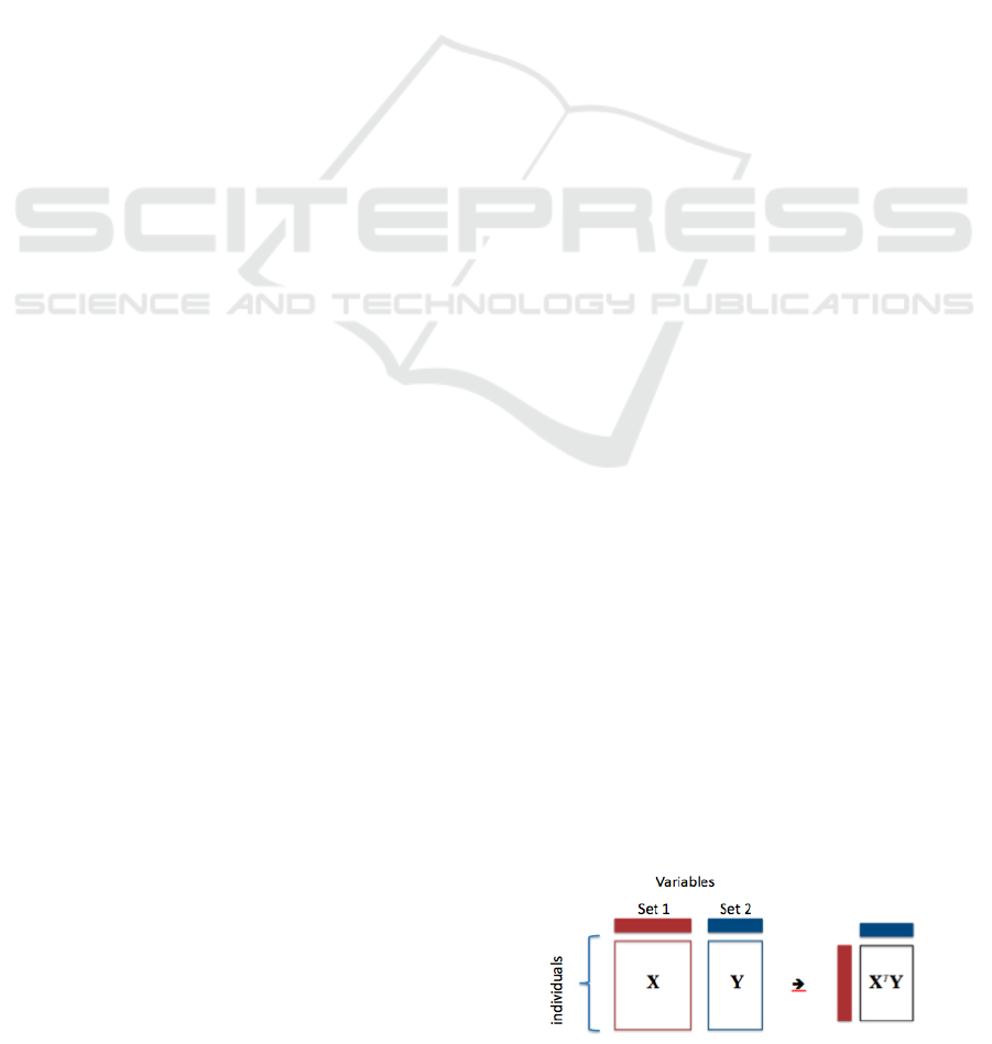
There are several strategies to match two data tables
namely the within and between principal components
analysis and the linear discriminant analysis. If two
tables are linked by the same individuals, one can find
a structure, a co-structure to study the relationship be-
tween the two set of variables.
Figure 1: Basic strategy to match two data tables.
Let’s call X and Y two continuous variables
280
Mukanahallipatna Simha S., Chau D. and Bremond F..
Feature Matching using CO-Inertia Analysis for People Tracking.
DOI: 10.5220/0004669502800287
In Proceedings of the 9th International Conference on Computer Vision Theory and Applications (VISAPP-2014), pages 280-287
ISBN: 978-989-758-009-3
Copyright
c
2014 SCITEPRESS (Science and Technology Publications, Lda.)

measured on the same individuals. Let’s call ¯x and ¯y
the means of X and Y respectively. Let’s call v(x) and
v(y) the descriptive variances of X and Y respectively.
A measure of the relationship between X and Y is
provided by the descriptive covariances:
cov(x, y) =
1
n
n
∑
i=1
(x
i
− ¯x)(y
i
− ¯y) (1)
The covariance can be negative or positive: that
depends on the sense of the relationship. All the
variance-covariance information can be gathered in a
matrix (which can be called the covariance matrix).
v(x) cov(x,y)
cov(y,x) v(y)
This matrix is symmetric: cov(x, y) = cov(y, x) and
cov(x, x) = v(x). One can divide the covariance be-
tween X and Y by the square roots of the variances of
X and Y (i.e., by the standard deviation of X and Y ).
By doing so, we obtain the coefficient of correlation
between X and Y .
cor(x, y) =
cov(x, y)
p
v(x)
p
v(y)
(2)
The closer the coefficient to either -1 or 1, the
stronger the correlation between the two variables.
The organization of this paper is as follows: after
the introduction, related work is discussed in section
2. Section 3 describes the Co-Inertia Analysis. The
proposed tracking system along with the algorithm is
presented in section 4. The experiments are reported
and discussed in section 5 followed by conclusion and
future work.
2 RELATED WORK
The typical feature matching techniques are Mean-
shift, Particle filter and Template matching. Mean
shift algorithm (Comaniciu et al., 2003) uses color
histogram to describe the target region for which the
amount of calculation needed is small resulting in
good real time implementation. But Mean shift al-
gorithm finds its disadvantage when the image is gray
scale or less textured and also when there is scale vari-
ations in the image. This results in losing the target
easily.
Particle filter (N.Johnson and D.C.Hogg, 1996)
for nonlinear filtering algorithm based on bayesian es-
timation has the unique advantage of processing the
parameter estimation. This algorithm does not find
its usage universally since it has a problem of conver-
gence besides being slow.
Template matching (Feng et al., 2008) is one of
the principle techniques in visual tracking. This algo-
rithm judges the matching degree based on the simi-
larity of the adjacent pixels. This calculation is easy
and fast but need to be calculated for the whole im-
age. Problem of this method occurs when the target is
deformed, rotated or occluded in which case it fails to
track the target.
The existing feature matching methods, besides
euclidean metric, includes the Matusita metric (Hager
et al., 2004), the Bhattacharyya coefficient (Comani-
ciu et al., 2003), the Kullback-Leibler divergence (El-
gammal et al., 2003), the information-theoretic simi-
larity measures (Viola and Wells., 1995), and a com-
bination of those (Yang et al., 2005). In (Jiang et al.,
2011) the author presents an adaptive metric into dif-
ferential tracking method where learning of optimal
distance metric is automatic for accurate matching. In
(Yang et al., 2005) the author describes about a new
similarity measure which allows the mean shift algo-
rithm to track more general motion models in an inte-
grated way using fast gauss transform leading to effi-
cient and robust non parametric spatial feature track-
ing algorithm.
The proposed method calculates the coefficient of
relationship between the physical objects in the cur-
rent frame to the physical objects in the previous
frame. This is enabled by getting the Histogram of
Oriented Gradients (HOG) features (Dalal and Triggs,
2005) of the physical objects in the first place and then
using COIA to find the coefficient of relationship be-
tween them for tracking the objects.
COIA has been used in Human computer interaction
and Biometrics community for finding audio-visual
speech synchrony (Goecke and Millar, 2003) (Eveno
and Besacier, 2005). For the first time we present
COIA as a feature matching technique of mobile ob-
jects for tracking in computer vision domain.
3 CO-INERTIA ANALYSIS
Coinertia analysis (COIA) is a relatively new multi-
variate statistical analysis for coupling two (or more)
sets of parameters by looking at their linear combi-
nations. It was introduced for ecological studies by
Doledec and Chessel (Doledec and Chessel, 1994).
As it appears to be relatively unknown in the Com-
puter Vision community, we will first give some back-
ground information. In COIA, the term inertia is used
as a synonym for variance. The method is related to
FeatureMatchingusingCO-InertiaAnalysisforPeopleTracking
281

other multivariate analysis such as canonical corre-
spondence analysis , redundancy analysis, and canon-
ical correlation analysis (CANCOR) (Gittins, 1985).
COIA is a generalization of the inter-battery analysis
by Tucker (Tucker, 1958) which in turn is the first step
of partial least squares (skuldsson, 1988).
COIA is very similar to CANCOR in many as-
pects. It also rotates the data to a new coordinate sys-
tem and the new variables are linear combination’s of
the parameters in each parameter set. However, here,
it is not the correlation between the two sets that is
maximized but the co-inertia (or co-variance) which
can be decomposed.
Compromise between the correlation and the vari-
ance in either set is found by COIA. It aims to find
orthogonal vectors - the co-inertia axes - in the two
sets which maximize the co-inertia value. The num-
ber of axes is equivalent to the rank of the co-variance
matrix. The advantage of COIA is its numerical sta-
bility. The number of parameters relative to the sam-
ple size does not affect the accuracy and stability of
the results (Doledec and Chessel, 1994). The method
does not suffer from co-linearity and the consistency
between the correlation and the coefficients are very
good (Dray et al., 2003). Thus, COIA is a very well
suited multivariate method in our case.
The co-inertia value is a global measure of the co-
structure in the two sets (mobile objects). The two
parameter sets vary accordingly (or inversely) if the
value is high and the sets vary independently if it is
low. The correlation value gives a measure of the
correlation between the co-inertia vectors of both do-
mains.
Furthermore, one can project the variance onto the
new vectors of each set and then compare the pro-
jected variance of the separate analysis with the vari-
ance from the COIA (see the appendix of (Doledec
and Chessel, 1994) for the theory). The ratio of the
projected variance from the separate analysis to the
variance from the COIA is a measure of the amount
of variance of a parameter set that is taken by the co-
inertia vectors. It is important to compare the sum
of axes, not axis by axis, because the variance pro-
jected onto the second axis depends on what is pro-
jected onto the first axis, and so on. Often it is suffi-
cient to look at the first 2-3 axes because they already
account for 90-95% of the variance. There are many
possibilities of giving inputs to COIA to find the rela-
tionship in general as described in (Dray et al., 2003).
Finally, a measure of overall relatedness of the two
domains, in our case mobile objects, based on the se-
lected parameters is given by the RV coefficient (Heo
and Gabriel., 1997).
In addition, COIA computes the weights (coeffi-
cients) of the individual parameters in the linear com-
bination’s of each set, so that it becomes obvious
which parameters contribute to the common structure
of the two sets and which do not. As has already been
pointed out, these weights are much more stable than
the weights in a CANCOR analysis. Finally, a mea-
sure of overall relatedness of the two domains based
on the selected parameters is given by the RV coeffi-
cient (Heo and Gabriel., 1997).
One of COIAs biggest advantages is that it can be
coupled with other statistical methods, such as corre-
spondence analysis and PCA. That is, these methods
are performed on the data of the two domains sepa-
rately and then a COIA follows. In fact, (Dray et al.,
2003) shows that seen in this context, COIA is a gen-
eralization of many multivariate methods. In our anal-
ysis, it means that we can use both shape PCs as input
for a COIA without being restricted as in the case of
CANCOR.
This multivariate method for finding the similarity
between two tables i.e two mobile objects between
frames in our case has been successfully tried and
showcased with effective results in comparison with
the state of the art.
3.1 Defining the Relationship between
Two Data Tables
Different statistics such as Pearson correlation co-
efficient or covariance can be used to measure the re-
lation between two variables. The purpose of this sec-
tion is to define a statistic that measures the relation
between two (or more) sets of variables. Let’s call
(X, Q
X
, D) a statistical triplet, where X is a dataset
containing p variables measured on n individuals. Q
X
and D represent the weights of the p variables and n
individuals, respectively. If all the variables of X are
centered, the inertia I
X
is the sum of variances. If D
is the diagonal matrix (n ×n) of individual weights
D = diag(w
1
, ....., w
n
) and if Q (p × p) is a metric of
this hyperspace, then inertia of the ”cloud of individ-
uals” around the reference point o is simply
I
o
=
n
∑
i=1
w
i
kX
i
−ok
2
Q
X
=
n
∑
i=1
w
i
kX
i
k
2
Q
X
(3)
In general
I
X
= trace(XQ
X
X
T
D) (4)
This total inertia is a global measure of the variabil-
ity of the data. It is the weighted sum of square dis-
tances measured with Q
X
, between the points of X (n
individuals) and the reference point o. If Q is the Eu-
clidean metric and D the diagonal matrix of uniform
weights and if o is the centroid of the cloud, the in-
ertia is simply a sum of variances. The individuals
VISAPP2014-InternationalConferenceonComputerVisionTheoryandApplications
282

X
i
can be projected on a Q
X
-normed vector u and the
projected inertia is expressed by
I(u) = u
T
Q
X
X
T
DXQ
X
u (5)
The total inertia can be easily decomposed on a set of
p orthogonal Q
X
-normed vectors u
k
:
I
o
=
p
∑
k=1
I(u
k
) =
p
∑
k=1
u
T
k
Q
X
X
T
DXQ
X
u
k
=
p
∑
k=1
kXQ
X
u
k
k
2
D
(6)
Let (Y, Q
Y
, D) be a statistical triplet, where Y is a
dataset containing q variables measured on n individ-
uals. Q
Y
and D represent the weights of the q vari-
ables and n individuals, respectively. If all the vari-
ables of Y are centered, the inertia I
Y
is the sum of
variances. In the same way as explained previously,
the inertia for this data will be
I
Y
= trace(Y Q
Y
Y
T
D) (7)
and can be decomposed as above on a set of vectors
v
k
and it is not difficult to study the common geome-
try of the two datasets. Co-Inertia is a global measure
of the co-structure of individuals in the two data hy-
perspaces. It is high when two structures vary simul-
taneously (closely related) and low when they vary
independently (not closely related). It is defined by
COI =
p
∑
k=1
q
∑
j=1
(u
T
k
Q
X
X
T
DY Q
Y
v
j
)
2
=
p
∑
k=1
q
∑
j=1
([X
k
]
T
DY
j
)
2
= trace(XQ
X
X
T
DY Q
Y
Y
T
D) (8)
If the datasets are centered, then inertia is a sum of
variances and co-inertia is a sum of square covari-
ances.
3.2 Principle of Co-Inertia Analysis
The co-inertia criterion measures the concordance be-
tween two data sets, and a multivariate method based
on this statistic has been developed. Co-inertia analy-
sis (Doledec and Chessel, 1994) is a symmetric cou-
pling method that provides a decomposition of the co-
inertia criterion on a set of orthogonal vectors. It is
defined by the analysis of the datasets defined. Dif-
ferent types of data lead to different transformations
(centering, normalization,...) of X and Y and to dif-
ferent weights Q
X
and Q
Y
. Co-inertia analysis aims
to find vectors v
1
and u
1
in the respective spaces with
maximal co-inertia. If X and Y are centered, then
COIA maximizes the square covariance between the
projection of X on u
1
and the projection of Y on v
1
:
P(u
1
) = (XQ
x
).u
1
cov
2
(P(u
1
), P(v
1
)) = corr
2
(P(u
1
), P(v
1
))
×var(P(u
1
)) ×var(P(v
1
)) (9)
This square covariance can be easily decomposed,
showing that COIA finds a compromise between the
correlation, the variance of individuals in their respec-
tive spaces viewpoint. The second and further pairs of
vectors (u
2
,v
2
...) maximize the same quantity but are
subject to extra constraints of orthogonality.
RV =
COI(X, Y )
p
COI(X, X)
p
COI(Y, Y )
(10)
The RV-coefficient is the coefficient of correlation
between the two tables X and Y . This coefficient
varies between 0 and 1: the closer the coefficient to
1, the stronger the correlation between the tables.
4 THE PROPOSED TRACKING
ALGORITHM
The proposed tracking algorithm needs a list of de-
tected objects in a temporal window as input. This
is enabled using a processing chain for image ac-
quisition, background subtraction (A.T. Nghiem and
Thonnat, 2009), classification, object detection and
tracking system (Chau et al., 2011). The size of the
temporal window is a parameter. This tracker system
first computes the link similarity between any two de-
tected objects appearing in a given temporal window
based on Co-inertia analysis. The trajectories that in-
clude a set of consecutive links from previous stages
are then computed to get the global similarity. Noisy
trajectories are removed through a filter.
To get the similarity link of the objects, first
Histogram of Oriented Gradients (HOG) (Dalal and
Triggs, 2005) descriptors of the detected physical ob-
jects in the current frame are calculated and compared
with the HOG descriptors of the detected Physical
Objects (PO) in the previous frame. This is where
the usage of COIA comes in to the picture. COIA is
used to compare the similarity between the physical
objects. For each detected object pair in a given tem-
poral window, the system computes the link similar-
ity (i.e. instantaneous similarity) defined using COIA.
A temporal link is established between these two ob-
jects when their link similarity is greater or equal to
a threshold. At the end of this stage, we obtain a
weighted graph (Chau et al., 2011) whose vertices are
the detected objects in the considered temporal win-
dow and whose edges are the temporally established
links associated with the object similarities.
FeatureMatchingusingCO-InertiaAnalysisforPeopleTracking
283
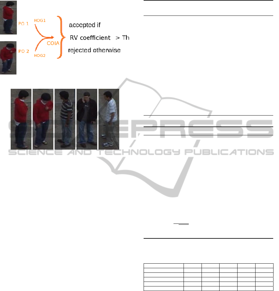
Figure 2: Physical Object (PO) similarity measure criteria.
Figure 3: From left PO1, PO2, PO3, PO4, PO5.
In this paper HOG descriptor is calculated on
the whole detected objects (whole bounding box) but
other possibilities are taking a patch in the detected
object and calculating HOG on the same for finding
similarity is also possible. Initial trial on finding fea-
ture similarity with color histograms between mobile
objects using COIA has been accomplished but will
be consolidated by combining different features for
efficiency and will be portrayed in future. Different
features like Local Binary Patterns, Local ternary pat-
ters etc. can be used as input to COIA.
As shown in Figure 2, the RV coefficient will be
higher for the same physical objects and lower for
the different physical objects which will enable us to
track the correct objects. The long term similarity
score between the object and the trajectory is calcu-
lated as explained in (Chau et al., 2011). To supple-
ment the frame to frame tracking and long term track-
ing, using COIA to measure the similarity between
mobile objects using HOG features, we make use of
dominant color, 2D distance, 2D shape ratio and 2D
area of the mobile objects as described in (Chau et al.,
2011) for better efficiency.
Table 1 signifies the behavior of COIA. In the Fig-
ure 3, PO1 and PO2 are same but with different poses
and the rest of the PO’s are different from PO1. As ex-
plained the HOG feature of each PO is calculated and
COIA is used to find the similarity between PO’s us-
ing the corresponding feature matrices. As expected,
the similarity between PO1 and PO2 should be higher
than any other PO combination from PO1. To sum-
Algorithm 1: Calculating F2F link between ob-
jects using COIA.
Require: Objects Detected from A Detector
1: function COMPUTEF2FCOIALINK(ObjectT,
imageT, imageTmN)
Check (objectT != NULL)
bboxTmN = Previous.getbbox;
bboxT = Present.getbbox;
ObjectTmN = getROI(imageTmN,bboxTmN);
ObjectT = getROI(imageT,bboxT);
ObjectTFeature = HOG(ObjectT);
ObjectTmNFeature = HOG(ObjectTmN);
COIAScore =
COIA(Ob jectTFeature, Ob jectT mNFeature);
return COIAScore;
Algorithm 2: Calculating COIA Score.
Require: Mobile Objects features matrices
function COIA(ObjectTFeature.matrix,
ObjectTmNFeature.matrix)
Check dimensions of the input matrices;
W = combine the two feature matrices;
[u,w,v] = SVD(W);
x = ObjectTFeature.matrix;
y = ObjectTmNFeature.matrix;
COI = trace(w);
Calculate I
x
from equation 4;
Calculate I
y
from equation 7;
RV =
COI
√
I
x
×I
y
;
return RV;
Table 1: Comparison of Histogram similarities (COIA, Cor-
relation, Intersection) and distances (Chi-square and Bhat-
tacharyya).
Algorithm PO1-PO1 PO1-PO2 PO1-PO3 PO1-PO4 PO1-PO5
COIA 1.0 0.8932 0.8663 0.7161 0.8429
Correlation 1.0 0.5532 0.2259 0.0287 0.2712
Intersection 1.0 0.8675 0.8585 0.7466 0.8212
Chi-square 0 0.2779 0.3746 0.8114 0.4584
Bhattacharyya Distance 0 0.1338 0.1564 0.2397 0.1738
marize COIA, Correlation and Intersection should be
higher for PO1-PO2 and lower for chi-square and
Bhattacharyya distance than others except PO1-PO1
obviously. The main motivation of Table 1 is to show-
case, for the first time in tracking mobile objects, that
COIA behaves as expected compared to other algo-
rithms in finding similarity between mobile objects.
All the values were calculated using OpenCV.
VISAPP2014-InternationalConferenceonComputerVisionTheoryandApplications
284

5 EXPERIMENTAL RESULTS
We present some real-time object tracking results us-
ing the proposed algorithm. The objective of this ex-
perimentation is to show the effectiveness of the pro-
posed algorithm in tracking system. People detec-
tion algorithm with Background subtraction based on
Mixture of Gaussian and Local Binary Pattern with
Adaboost is used for detection.
HOG descriptor of the OpenCV is used to get
the features of the detected objects which goes as in-
put to the COIA routine to calculate the coefficient
of relationship between them. The videos used for
testing the tracker belongs to a public benchmark
dataset ETISEO (Etiseo, ) and private dataset Hospi-
tal. The algorithm has been implemented in C++ but
was coded in Matlab initially to verify the proposed
idea. The proposed method runs on Intel Xeon 8 core
2GHz CPU.
In order to evaluate the tracking performance, we
use the three tracking evaluation metrics defined in
the ETISEO project (Etiseo, ). The first tracking eval-
uation metric M1 measures the percentage of time
during which a reference object (ground truth data)
is correctly tracked.
The second metric M2 computes throughout time
how many tracked objects are associated with one ref-
erence object. The third metric M3 computes the
number of reference object IDs per tracked object.
These metrics must be used to obtain a complete per-
formance evaluation. The metric values are defined in
the interval [0, 1]. The higher the metric value is, the
better the tracking algorithm performance.
All the result images shown contains green bound-
ing box representing tracking of the person associated
with id and blue ellipse shows the person with track-
ing/trajectory path of the person.
The Figure 5 shows the tracked image sequences
of Hospital dataset. This dataset is challenging in
terms of shadow and pose change of the object (per-
son). The proposed algorithm for tracking produces
a perfect tracking through out the video sequence as
mentioned in Table 2. Figures 6, 7 and 8 illustrates the
tracking of objects for ETISEO public dataset video
sequence. This dataset is very challenging because of
many illumination/contrast changes in the frames.
Table 2: Tracking results of two video sequences - Figure 5
and 7.
Dataset M1 M2 M3
Hospital 1.0 1.0 1.0
ETISEO 1.0 1.0 1.0
As shown in Figure 6, the video sequence is of
low light settings and there are transitions from light
switched off to on and vice-versa which makes the
tracking very challenging. The proposed algorithm
for tracking again produces perfect tracking results
for this video sequence in-spite of challenging light-
ing/contrast conditions. The results are shown in Ta-
ble 2.
The contrast of an object is defined as the color in-
tensity difference between the object and its surround-
ing background. Figure 4 shows the tracking result in
the sequence ETI-VS1-BC-13-C4 (from the ETISEO
dataset) at some frames in two cases: the first row il-
lustrates the tracking result using the proposed COIA
method; the second row illustrates the tracking result
using (P.Bilinski et al., 2009). From frame 1400 to
frame 1425, the object contrast does not change and
the tracking results are good in both cases. From
frame 1425 to frame 1525, the object contrast de-
creases, and from frame 1525 to frame 1600 it in-
creases. While the proposed COIA based tracker still
ensures a good performance during these two periods,
the (P.Bilinski et al., 2009) tracker cannot keep good
tracking result. When the object contrast changes, the
distance between HOG features of the physical ob-
jects in (P.Bilinski et al., 2009) decreases and hence
tracking fails (change in bounding box color). So the
variation of object contrasts influences the tracking
performance.
Table 3: Tracking results of ETI-VS1-BE-18-C4 sequence
- Fig 8.
Metric Proposed method T1 T8 T11 T12 T17 T22 T23
M1 0.6 0.48 0.49 0.56 0.19 0.17 0.26 0.05
M2 1.0 0.8 0.8 0.71 1.0 0.61 0.35 0.46
M3 1.0 0.83 0.77 0.77 0.33 0.80 0.33 0.39
In these experiments, tracker results from seven
different teams (denoted by numbers) in ETISEO
(Video understanding Evaluation) project (Etiseo, )
have been presented: T1, T8, T11, T12, T17, T22,
T23. Because names of these teams are hidden, we
cannot determine their tracking approaches. Table 3
presents performance results of the considered track-
ers. The tracking evaluation metrics of the proposed
tracker gets the highest values in most cases compared
to other teams.
Table 4: Tracking result comparison of PETS sequence -
Fig 9.
PETS2009view001 MOTA MOTP
(Berclaz et al., 2011) 80.00 58.00
(Shitrit et al., 2011) 81.46 58.38
(Andriyenk and Schindler, 2011) 81.84 73.93
(Henriques et al., 2011) 84.77 68.74
Proposed method 88.42 65.60
FeatureMatchingusingCO-InertiaAnalysisforPeopleTracking
285
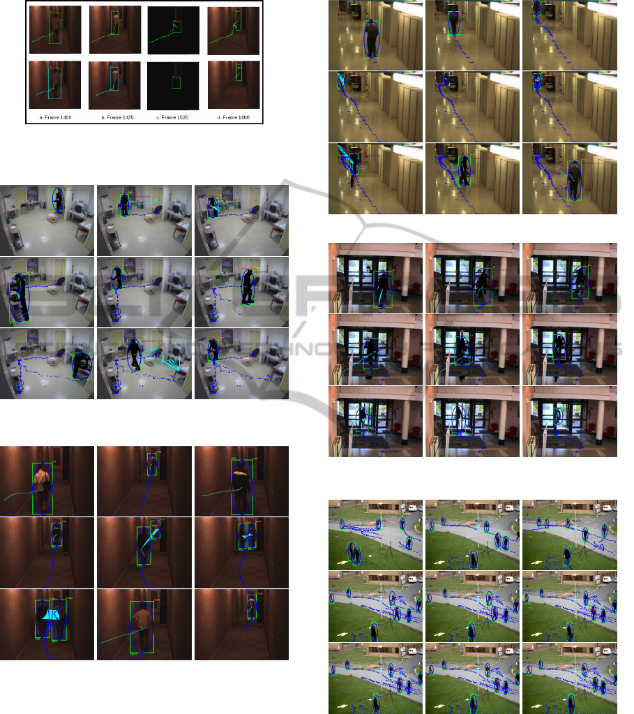
Figure 4: Top row proposed tracking algorithm in this
paper, bottom row tracking result from (P.Bilinski et al.,
2009).
Figure 5: Tracking of a patient in the hospital video se-
quence.
Figure 6: People Tracking in the ETISEO ETI-VS1-BC-13-
C4 video sequence.
In Table 4 (Zamir et al., 2012) Standard CLEAR
MOT (Kasturi, 2009) has been used as evaluation
metrics. MOTA (Motion Object Tracking Accu-
racy) measures False positives, false negatives and
ID-Switches . The average distance between the
ground truth and estimated target locations has been
defined as MOTP (Motion Object Tracking Preci-
sion). MOTP signifies the ability of the tracker in es-
timating the precise location of the object, regardless
of its accuracy at recognizing object configurations,
Figure 7: People Tracking in a ETISEO video sequence.
Figure 8: People Tracking in the ETISEO ETI-VS1-BE-18-
C4 video sequence.
Figure 9: People tracking on PETS View-001-S2L1 video
sequence.
keeping consistent trajectories, and so forth. There-
fore, MOTA has been widely accepted in the liter-
ature as the main gauge of performance of tracking
methods. Video sequence View-001-S2L1 Figure 9
from PETS 2009 dataset has been used to compare
the proposed tracking method with other tracking al-
gorithms.
VISAPP2014-InternationalConferenceonComputerVisionTheoryandApplications
286

6 CONCLUSIONS AND FUTURE
WORK
This paper presents a new approach to track physi-
cal/mobile objects, for the first time in this domain,
using COIA which measures the similarity between
them. The proposed method has been successfully
validated with public datasets as mentioned in the
previous section and shows promising results. This
method has been validated with challenging video se-
quences to show the significance of the approach. We
propose to use other features like color histograms,
Local Binary Patterns etc. and combination of multi-
ple features for the detected objects to find the similar-
ity between them using COIA. We would also like to
propose in future to come up with a different weight-
ing strategy for the features of the objects in finding
the similarity using COIA.
REFERENCES
Andriyenk, A. and Schindler, K. (2011). Multi-target track-
ing by continuous energy minimization.. CVPR.
A.T. Nghiem, F. B. and Thonnat, M. (2009). ”Controlling
Background Subtraction Algorithms for Robust Ob-
ject Detection”. ICDP.
Berclaz, J., Fleuret, F., Turetken, E., and Fua, P. (2011).
Multiple object tracking using k-shortest paths opti-
mization.. TPAMI.
Chau, D., Bremond, F., and Thonnat, M. (2011). A multi-
feature tracking algorithm enabling adaptation to con-
text variations. 4th International Conference on Imag-
ing for Crime Detection and Prevention 2011 (ICDP
2011), pages P30–P30.
Comaniciu, D., Ramesh, V., and Meer., P. (2003). Kernel-
based object tracking. TPAMI, 5(25):564–577.
Dalal, N. and Triggs, B. (2005). Histograms of oriented
gradients for human detection. CVPR, 1:886 –893 vol.
1.
Doledec, S. and Chessel, D. (1994). Co-inertia analysis: an
alternative method for studying species-environment
relationships. Freshwater Biology, 1:277–294.
Dray, S., Chessel, D., and Thioulouse, J. (2003). Co-inertia
analysis amd the linking of ecological tables. Ecology.
Elgammal, A., Duraiswami, R., and Davis., L. S. (2003).
Probabilistic tracking in joint feature-spatial spaces.
CVPR, 1:I–781–I–788.
Etiseo. ”http://www-sop.inria.fr/orion/ETISEO/”.
Eveno, N. and Besacier, L. (2005). A speaker independent
liveness test for audio-video biometrics. 9th European
Conference on Speech Communication and Technol-
ogy, pages 232–239.
Feng, Z. R., Lu, N., and Jiang, P. (2008). Posterior probabil-
ity measure for image matching. Pattern Recognition,
41:2422–2433.
Gittins, R. (1985). Canonical Analysis. Springer-Verlag,
Berlin, Germany,.
Goecke, R. and Millar, B. (2003). Statistical Analysis of
the Relationship between Audio and Video Speech Pa-
rameters for Australian English. AVSP.
Hager, G. D., Dewan, M., and Stewart., C. V. (2004). Mul-
tiple kernel tracking with ssd. CVPR, 1:I–790–I–797.
Henriques, J., Caseiro, R., and J., B. (2011). Globally op-
timal solution to multi-object tracking with merged
measurements.. ICCV.
Heo, M. and Gabriel., K. (1997). A permutation test of as-
sociation between configurations by means of the RV
coefficient,. Communications in Statistics - Simula-
tion and Computation,, 27:843–856.
Jiang, N., Liu, W., and Wu, Y. (2011). Adaptive and dis-
criminative metric differential tracking. CVPR 2011,
pages 1161–1168.
Kasturi, R. (2009). Framework for performance evalua-
tion of face, text, and vehicle detection and tracking
in video: Data, metrics, and protocol.. TPAMI.
N.Johnson and D.C.Hogg (1996). Learning the distribution
of oject trajectories for event recognition. Image and
Vision computing, 14:583–592.
P.Bilinski, F.Bremond, and M.Kaaniche. (2009). Multi-
ple object tracking with occlusions using HOG de-
scriptors and multi resolution images.. ICDP, London
(UK),.
Shitrit, H., Berclaz, J., Fleuret, F., and P., F. (2011). Track-
ing multiple people under global appearance con-
straints.. ICCV.
skuldsson, A. H. (1988). Partial least square regression.
Journal of chemometrics, 2:211–228.
Tucker, L. (1958). An inter-battery method of factor analy-
sis. Psychometrika, 23:111–136.
Viola, P. and Wells., W. M. (1995). Alignment by maxi-
mization of mutual information. ICCV, page 0:16.
Yang, C., Duraiswami, R., and Davis., L. (2005). Effi-
cient mean-shift tracking via a new similarity mea-
sure. CVPR, 1:176–183.
Zamir, A. R., Dehghan, A., and Shah, M. (2012). Gmcp-
tracker: Global multi-object tracking using general-
ized minimum clique graphs. ECCV.
FeatureMatchingusingCO-InertiaAnalysisforPeopleTracking
287
