Low-Discrepancy Distribution of Points on Arbitrary Polygonal
3D-surfaces
Alena Bulyha, Wolfgang Herzner, Markus Murschitz and Oliver Zendel
Safety & Security Department, AIT Austrian Institute of Sciences,
Donau-City-Straße 1, 1220 Vienna, Austria
Keywords: 3D-surfaces, Geometric Discrepancy, Halton Sequences, Hammersley Sequences, Low-Discrepancy, Sam-
pling, Segmentation, Uniform Distribution, Unfolding, Wrapping.
Abstract: This paper presents a technique for automatic distribution of points on 3D-surfaces that are defined as
meshes of polygons (usually triangles) such that the distribution has a low discrepancy. The work is moti-
vated by the quest for representing arbitrary 3D-objects by a minimal number of surface points such that dif-
ferent views and arbitrary occlusions of objects can be effectively distinguished by simply using the visible
surface points. The approach exploits low-discrepancy sequences on the unit square such as those proposed
by Hammersley or Halton.
1 INTRODUCTION
In computer graphics, a standard technique for mod-
elling the geometry of 3D-objects is to represent
their surface as polygon meshes, mostly consisting
of triangles. The question we want to address in this
work is: how to distribute points on a polygonal
mesh of a 3D-object such that for each possible view
(2D-projection) of the object, the visible fraction of
points can be used as representative for the visible
fraction of its total surface in that view? Of course,
for economic reasons the question should be extend-
ed by “with as few points as possible”.
A hint for a possible answer can be found in 2D-
geometry. Consider you want to distribute a set P of
n points on a square U such that for any sub-area R
U, larger than some given minimum, the ratio of
points contained in R to n is as close as possible to
the ratio of the areas of R and U; i.e. the number of
points found in R can be used as a good approxima-
tion for the size of R relative to U. It turns out that
both regular and random distributions are not well
suited for that purpose, while in the case of continu-
ous uniform distributions, the local point density is
proportional to the surface area covered by these
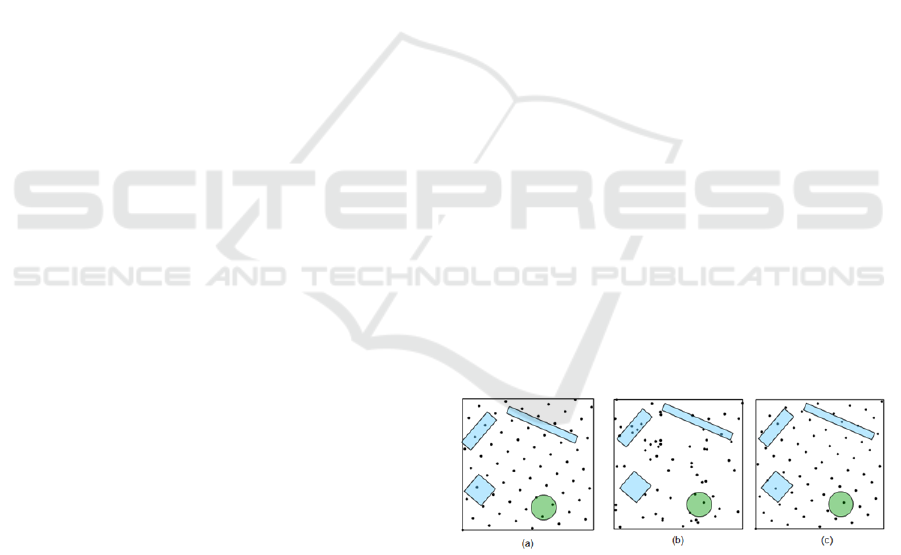
points. This is illustrated in Figure 1.
The measure for the deviation between the real
size and that indicated by the number of covered
points is called geometric discrepancy (see chapter 2
for precise definitions and more background). Evi-
dently, the smaller this value the better.
Figure 1: Point distribution examples on a square: (a) the
points arranged in a lattice; (b) random (Monte Carlo)
points; (c) Hammersley points.
Actually, low-discrepancy point sets have been
widely used in computer graphics and image pro-
cessing for point based object representation (Quinn
et al., 2007), for improving image quality (Wong et
al., 1997), for the purpose of antialiasing (Wand and
Straßer, 2003), for half-toning (Hanson, 2003) or for
illumination (Dachsbacher and Stamminger, 2006).
Several methods for producing low-discrepancy
sequences on the unit square have been proposed by
Hammersley (Hammersley, 1960), Halton (Halton,
1960), Sobol (Sobol, 1967), Niederreiter (Nieder-
reiter and Chao, 1995) and have been further inves-
tigated by other scientists or research groups (Cheng
and Druzdzel, 2000, Grabner et al., 2012).
This work addresses uniform distribution of
points on arbitrary polygonal 3D-surfaces. The idea
79
Bulyha A., Herzner W., Murschitz M. and Zendel O..
Low-Discrepancy Distribution of Points on Arbitrary Polygonal 3D-surfaces.
DOI: 10.5220/0004659900790087
In Proceedings of the 9th International Conference on Computer Graphics Theory and Applications (GRAPP-2014), pages 79-87
ISBN: 978-989-758-002-4
Copyright
c
2014 SCITEPRESS (Science and Technology Publications, Lda.)

is to unfold the polygon resulting in a 2D- represen-
tation, then to place low-discrepancy distributed
points on it, and finally, to map these placements
back to the 3D object. The discrepancy is treated in
this work only analytically. To control the quality of
the performed technique, the irregularity measure as
a comprehensible geometric interpretation is pre-
sented and is explained by the algorithm and several
examples. The proposed approach concentrates only
on triangular meshes. However, the method could
also be extended for surfaces represented by arbi-
trary polygons.
This paper is structured as follows. In the next
section, similar work found in literature is shortly
discussed, while Section 3 introduces the mathemat-
ical background of geometric discrepancy. Section 4
describes our method and its evaluation criteria.
Section 5 presents and discusses some application
examples and Section 6 draws a conclusion.
2 RELATED WORK
Previous research in the area of sampling techniques
mainly concentrated on uniform scattering of points
on planar domains (Pillards and Cools, 2005, Hofer
and Pirsic, 2011) and on spherical surfaces (Rakh-
manov et al., 1994, Cui and Freeden, 1997).
More recent investigations address low-
discrepancy point distributions on an arbitrary sur-
face. They include different sampling strategies
based on uniform distribution of lines in the 3D
space, on space filling curves. For instance, Quinn
(Quinn et al., 2007) use Hilbert curves to fill param-
eterized meshes and map them onto the surface. The
low-discrepancy sampling happens along the Hilbert
curves. The parameterization methods are based on
solving the sparse linear system and can be applied
only to surface-sections that are homeomorphic to a
disk. Thus, the pre-processing step is also applied to
cut an arbitrary mesh into a set of topological disks
and to generate the Hilbert curves. Because the
choices of parameterization and cutting algorithms
have little effect on the final sampling due to the
adaptive nature of the Hilbert curve and
the re-
meshed surface of the object can be slightly changed
during this process, the Hausdorff distance is used to
assess how well the new shape is preserved. Our
approach, however, is shape accurate and is easy to
implement. The initial mesh is not changed when
providing the low-discrepancy distribution over the
planar domain and mapping it back to the original
surface.
Rovira (Rovira et al., 2005) suggest a sampling
technique based on intersecting of lines uniformly
distributed in 3D-space with polygonal models.
Several algorithms to generate the set of uniformly
distributed lines are proposed. Each of them utilizes
the low-discrepancy point set in four dimensions and
is based on the approximation of a binomial distribu-
tion by a Poisson distribution. Such approximation is
only suitable for large number of lines. Thus, the
proposed approach causes the large number of uni-
formly distributed lines and, therefore, the large
number of intersecting points. In contrast, using the
scattering of the 2D low-discrepancy points set onto
the surface our algorithm can deal with a small
number of sampling points.
Our approach is also related to prior works on
mesh segmentation and mapping the segments onto
a planar domain (also called mesh unwrapping or
unfolding). The partitioning techniques of boundary
meshes is often application dependent. In fact, it can
be distinguished between two general types: seg-
mentation of the whole object into meaningful, vol-
umetric parts and partitioning of the surface mesh
into segments under some criteria. A detailed over-
view of these methods is given in (Shamir, 2008).
The work described in this paper does not concern
optimal segmentation, but a simple unfolding algo-
rithm has been designed to fulfil the given goals.
3 MATHEMATICAL
BACKGROUNDS
Let P be a set of n
U
points that are distributed on the
unit square U=[0,1)[0,1).
Collection S
2
is the set of sampling figures on
the unit square U. In general, it can be any set con-
sisting of scaled and translated copies of fixed poly-
gons or polytopes (Matousek, 1999 p.10). Therefore,
S
2
can include such sample figures F which contain
the unit square or some part of it or do not overlap
with U. As only overlap with U is of interest, the
collection shall be reduced to the set { R | R=F∩U}.
Without any further notation, let R be an element
from collection S
2
and R U.
N(R) is the number of points of P within R and,
therefore, N(U)=n
U
. The geometric discrepancy D
for the unit square U can be defined (Matousek,
1999, p.13, Alexander, 2004, p.283) by taking a
norm of the difference between the actual number of
points within any sampling figure R and the ex-
pected number of points hitting R, i.e.
D
U,P,
,
≔
‖
‖
,
((1)
GRAPP2014-InternationalConferenceonComputerGraphicsTheoryandApplications
80
where ∈
. vol(R) denotes the area of R, as frac-
tion of U, i.e. vol(R):=area(R)/area(U), and
is the expected number of points hitting
R. The function ∆
is de-
noted as discrepancy function with the following
norm:
‖
∆
‖
∆
,1
, (2)
‖
∆
‖
∞
sup
∈
|
∆
|
,..
; (3)
Let
d
m
:=1/n
U
be the mean distance between clos-
est neighbour points, where
n
U
=#P is the cardinali-
ty of
P that is equal to the prescribed density.
In our work we use the Hammersley or Halton
sequences to calculate the potentially infinite uni-
formly distributed sequence W on the unit square,
and utilize the first n points to build the set P. These
sequences are based on radical inversion and modi-
fications of this inversion (Halton, 1960, Hammers-
ley, 1960). The sequences are defined in an arbitrary
number of dimensions. An implementation of them
is described in (Wong et al., 1997).
For every natural number n, the discrepancy for
both Hammersley or Halton sequences is bound, i.e.
there is an absolute positive constant c such that
|
D
U,P,
,∞
|
|
log
|
, where S
2
S
r
is a set
of axis-parallel rectangles (Matousek, 1999, p.41).
We can also say in this case that the discrepancy
satisfies D
U,P,S
,∞
log
.
If S
2
S
d
is a set of two-dimensional disks of ra-
dius r, and n=#P, then there are two absolute posi-
tive constants c
1
and c
2
(Alexander, 2004, theorem
13.3.6) that depend on the radius. The discrepancy
can be estimated as follows:
⁄
D
U,P,S
,∞
⁄
log
(4)
Some further discrepancy estimations are also
given in (Alexander, 2004, Berg, 1996, Chen and
Travaglini, 2007).
Because the estimation of the discrepancy de-
pends on the collection S
2
and used norm, we further
assume that the collection is a set of different convex
figures and is large enough; and the lower and upper
bounds of discrepancy exist:
#
D
U,P,
,L
#
. (5)
As already mentioned in the introduction, we
want to distribute points on 3D-surfaces by unfold-
ing their meshes, mapping them to U, and re-
mapping the “caught” points of P back to the sur-
face.
If we apply only rotation, translation and iso-
tropic scale for the mapping between planar surface
elements and U, the transformed set of points is also
uniformly distributed with only minor change in the
discrepancy, see also concept of isotropic discrepan-
cy in (Matousek, 1999).
To measure the discrepancy D
O
,Q,S
,
of
the points set Q on the surface of a 3D-object, a
feasible collection S
OM
of the sample figures should
be selected. The collection proposed in (Quinn et al.,
2007) is a sub-set of the triangulated object’s mesh
(OM or O
M
) that is chosen as “a contiguous set of
triangles, grown from a random seed triangle to a
random number of triangle rings”. The mesh seg-
ments with random number of triangles could also
be used instead of the ring of triangles.
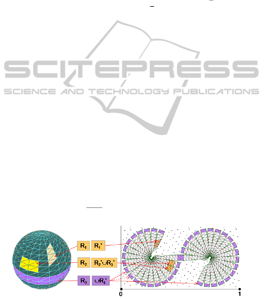
As an example, consider some sphere with set of
points Q={q
i
} scattered over its surface. The sphere
is scaled in such a way that its unfolded mesh is
measure-preserving mapped to the unit square, as is
shown in Figure 2, where the mapped points
Q={q
i
}O
M
and the initial points Q
*
={q
i
*
} U are
given in red colour.
The part of the unit square, which is not covered
by the unfolded mesh, is completed with points
Q
={q
i
}, i.e. P
*
= Q
Q
*
, P
*
U. The points Q
are shown in Figure 2 in black colour.
Figure 2: Example of the discrepancy calculation on the surface of a 3D-object.
Low-DiscrepancyDistributionofPointsonArbitraryPolygonal3D-surfaces
81

Let S
OM
*
={R
i
*
} be the set of the unfolded sample
figures. For instance, in the given example the sam-
ple figure R
1
is unfolded to R
1
*
, the
figure R
2
is un-
folded to convex figures R
2
*
and R
3
*
and the unfold-
ed figure R
3
is the set of triangles pairs R
k
*
.
Assume also that the set S
OM
*
is reasonably ex-
tended to S
2
*
and used to measure the discrepancy of
P
*
in the unit square, i.e. S
OM
*
S
2
*
and
#P
∗
DU,P
∗
,
∗
,L
#P
∗
. Thus, each
discrepancy function calculated in the unit square
has an upper bound ∆
∗
#P
∗
, ∀
∗
∈
∗
.
Consider the discrepancy function calculated for
the set of points on the spherical surface. Because
isotropic mapping is used, the expected number of
points and the real one inside the sample figure will
not change after unfolding and, therefore, the dis-
crepancy function of R
1
is ∆
∆
∗
, where
R
1
S
OM
and R
1
*
S
2
*
. For the sample figure R
1
S
OM
the discrepancy function is calculated as (R
2
) =
(R
2
*
) + (R
3
*
) .
The strongest influence on the discrepancy
D
O
,Q,
,
is given by a sample figure like
R
3
S
OM
, i.e. ∆
∑
∆
∗
,
39. The
influence of the sample figures
∗
on the discrepan-
cy decreases with increased density of distributed
points, i.e. with increase of the cardinality of Q. For
each
∗
there exists an absolute positive constant
#
1, such that each discrepancy function
∗
is smaller than
#P
∗
by the factor of
#
, i.e. ∆
∗
#
#P
∗
, where k
i
f
i
. Therefore,
‖
∆
‖
∑
#
#P
∗
max
#
#P
∗
,
(6)
where R
i
S
OM
f
d
=max{ f
i
}.
The unfolded sample figure is decomposed into a
maximum of f
d
compact convex parts/bodies. f
d
is
called decomposition degree and depends on object
shape and its unfolding. In this example, f
d
=39.
Thus, the discrepancy can be estimated as fol-
lows:
D
O
,Q,
,
#
#P
∗
,
(7)
where c(#Q) 1 is inversely proportional to the
density as well.
Thus, the discrepancy on the surface of the 3D-
objects could be compared under the assumptions
stated above with the discrepancy of the points dis-
tributed on the unit square.
Hence, the discrepancy D
O
,Q,S
,
calcu-
lated over the total object mesh depends on the de-
composition degree in the case of small points set; if
the point set Q has the cardinality significantly larg-
er than f
d
, the decomposition degree f
d
does not have
a major impact on the discrepancy. Note also, that
the discrepancy could be exactly equal to
#P
∗
on some local parts of the surface.
Such dependency of discrepancy on size and
shape of the test figures containing the respective
uniformly distributed point sets is investigated in
detail in the next section.
4 ALGORITHMS
In order to minimize the geometric discrepancy over
the whole surface, the triangles should be assembled
to as large as possible segments while retaining the
original neighbourhood of the triangles.
To distinguish between 3D and 2D domains, we
denote a (connected) subsection of a triangulated
surface as segment and its unfolded (flattened) coun-
terpart as strip. The effect of discrepancy increase
not only applies to edges where segments touch, but
everywhere along their edges where their 2D projec-
tions are split with a distance smaller than mean
distance d
m
. A similar effect is caused by the in-
verse, namely when parts of segments mapped to a
strip overlap in a zone up to width d
m
. These effects
are illustrated in Figure 3. Interstices may likely
appear when a polygon mesh representing a curved
surface like that of a sphere is flattened; see Figure 2
for an example. The elongated parts of a strip be-
tween interstices are denoted as “fingers”. If fingers
extend over saddle regions in the segment, they may
overlap in the strip. In general, the zone of width d
m
along the edges of a strip contributes most to the
increase of discrepancy, because here the continuity
of the point distribution as taken over from unit
square U is broken whenever it touches another
border.
Figure 3: Zones of the strip with larger discrepancy in
interstices (left) and overlaps (right). Because the points in
overlap regions are mapped to multiple segments, the
distances between their copies on the 3D-surface would be
smaller than d.
GRAPP2014-InternationalConferenceonComputerGraphicsTheoryandApplications
82

Following these observations, the minimization of
the “irregular border zone” A can be achieved by
following goals:
Maximize size of segments.
Minimize ratio edge length / area of strips.
Minimize elongation of strips.
Minimize concave zones.
Minimize number of strips and, therefore, the de-
composition degree of the sample figures.
Planes should not be split.
Optimizing all goals with a single algorithm is
difficult if not impossible. This approach will focus
on achieving a good balance between these require-
ments.
4.1 Mesh Segmentation and Unfolding
The simple segmentation-unfolding algorithm we
are using works as follows:
1) Find the 2D skeleton of the (first) strip:
Starting with the triangle T
l
(e
i
(v
i
,v
j
), e
j
(v
j
,v
k
),
e
k
(v
k
,v
i
)) with the largest edge, e.g. e
i
(v
i
,v
j
), its or-
dered set of vertices is congruently mapped to the
plane. The triangle T
l
and vertex v
i
are saved in cor-
responding look-up tables with a mark “is mapped”.
The next triangle T
l+1
that is chosen is the one at-
tached to the longest of the remaining mapped edg-
es, e.g. v
r
, of the previous triangle; and its non-
considered vertex is also mapped to the plane, in the
same way as vertex v
k
. The triangle T
l+1
and vertex
v
r
are saved in corresponding look-up tables with
mark “is mapped” as well. The process continues
until a chosen triangle has already been mapped.
If the longest edge of the start-triangle has a non-
mapped adjacent triangle, the process can be pur-
sued in the other direction. When no more triangles
can be added to the strip, the ordered sequence of
outer edges is saved as strip-boundary.
2) In the next step, the algorithm moves along
the strip-boundary and adds to the strip those trian-
gles which were not yet added to any strip and
which, together with their neighbours from the seg-
ment, establish a plane or ”almost” a plane, i.e. the
minimal angle between them is closed to 180°. By
adding the new triangle to the strip, the correspond-
ing boundary edge is replaced by the new edges.
3) Next, we look once more along the boundary
to find such leftover triangles that are not yet
mapped but are surrounded by unfolded segments.
4) If the cardinality of the strip is smaller than a
given threshold, the strip will be allowed to grow
again along its boundary, and the steps 2 and 3 will
be repeated as long as possible.
5) The accumulation of the next segment and
strip starts from the largest edge of the saved strip-
boundaries.
The unfolding of the segments onto the plane
does not change the area or the geometry of the
individual triangles but creates splits and overlap-
ping regions inside or at the border of the strips.
As already mentioned, even tiny gaps can lead to
missing sampling points and very small overlapping
can cause doubling of points, which both increase
the discrepancy. One source of such regions is float-
ing-point operations, because when performed in
different orders they do not always lead to exactly
the same result. The second one is the roughness of
the object surface. In our approach we extract and
handle thin interstices and thin overlaps using a
correction algorithm (see Section 4.2).
4.2 Low-discrepancy Points Wrapping
The distribution of points on the arbitrary surface is
operated in the following manner:
1) The strips generated with the algorithm de-
scribed before are mapped to a planar domain.
2) Points are scattered on the planar domain that
contains the strips. The cardinality of the points set
depends of the area of the planar domain and some
default density. The default density can be given, for
instance, by the user. Because used algorithm gener-
ates points in the unit square, the set of points need
to be isotropic scaled to the planar domain.
3) The strips are positioned on the planar do-
main, using another low-discrepancy set of points
with cardinality that is equal to the number of strips.
4) The total area of “irregular zones” is calculat-
ed for the whole object. If the irregularity ratio, i.e.
the ratio of the area of “irregular zone” to the total
surface area (see Section 4.3), is larger than a given
threshold, the used point density is increased (and
hence the mean distance d
m
between neighbours
decreased). All points inside each planar triangle are
mapped back to the 3D-surface.
5) The points inside thin interstices and thin
overlaps are mapped to the corresponding edges
using the following correction algorithm:
a) For each strip find thin interstices and thin
overlapping regions. A region width of 0.1 d
m
is
used in the examples below;
b) If the interstice contains a point, project it or-
thogonally onto the closest edge;
c) If the overlapping contains a point, find all
corresponding points on the 3-D surface and remove
all copies but one.
Low-DiscrepancyDistributionofPointsonArbitraryPolygonal3D-surfaces
83

The next section describes how the accuracy of
the approach is estimated by the using of irregularity
ratio.
4.3 Unfolding Accuracy
Let R be the irregularity ratio R=A/A
tot
, where A
tot
is the total surface area of the object and A is the
area of the “irregular zone”. A=A(b) is estab-
lished along each boundary edge b. Besides d
m
, the
boundary length and the shape of the strip where b
belongs influence A(b) as well.
The area of the irregular zone can be calculated
exactly for simple objects. For complex objects, we
establish A for each strip, where the boundary
consists of a sequence of ordered edges: {e
1
, … , e
j-1
,
e
j
, e
j+1
, e
Ne
}, where N
e
is the number of boundary
edges of a strip and edges e
1
and e
Ne
are neighbours.
A rough estimate of A can be calculated as fol-
lows:
∆
∑
len
2
, (8)
where len
is the length of the edge e
j
and
is a number of concave strip vertices.
To calculate a more precise estimation of value
for A, the following cases could be considered:
a) the “irregular zone” adjacent to e
j
is a triangle;
b) the “irregular zone” adjacent to e
j
is a rectan-
gle, avoid in this case that some areas do not calcu-
lated twice;
c) at least one of the half-angle between the edg-
es adjacent to e
j
is larger than 90°, the corresponding
corner of the “irregular” trapezoid or parallelogram
could be reduced to a circular sector.
The whole value of A is accumulated along the
boundary of the strip. Note, that the irregular area
within thin “fingers” or zones with a width < 2 d
m
could be calculated twice. In our approach we do not
search for such overlaps but use them to weight the
irregularity ratio if the strip has unwanted thin “fin-
gers” or zones. Therefore, in some cases the ratio R
can be larger than 1.
An important concept in computer graphics is
that of level-of-detail (LoD): a prescribed resolution
depending on the distance between camera and the
object (more precisely, some fixed point of the ob-
ject, e.g. its centre). Evidently, calculated points set
with large R can be effectively used at large LoD to
estimate the visible surface fraction. In general, the
balance between the irregularity ratio and density
should be deciding for each LoD.
5 EXPERIMENTAL RESULTS
AND DISCUSSION
The low-discrepancy points wrapping approach is
tested by using the different surface meshes, includ-
ing meshes of geometrically simple objects (Figure
4), analytically calculated meshes (Figure 5), and
meshes which are produced by a laser scanner with
adaptive re-meshing (Figure 7) and without re-
meshing (Figure 6). Such meshes do not only differ
in topology and in the number of connected compo-
nents, but some of them are also not optimized to
achieve a regular and/or structured grid.
Figure 4 shows the scattering of points onto a
sphere. The mesh has a structured curvilinear grid.
The segmentation algorithm yields one segment, of
which the two-dimensional projection (Figure 4e)
has many tiny interstices. The points provided by the
correction algorithm are shown in Figure 4f in pink
colour. To achieve the irregularity ratio of 0.95, 770
points shall be scattered, while the distribution of the
192 points leads only to irregularity of R=1.32.
By using the Hammersley algorithm in the spherical
coordinates (Wong et al., 1997) we can also calcu-
late the low-discrepancy points set distributed direct-
ly onto the spherical surface and compare them with
our approach, see Figures 4a and 4b versus 4c and
4d, respectively.
In the next example the low-discrepancy points
wrapping approach is applied to an object created
analytically by a cup-generator, the object is shown
in Figure 5. The mesh has a block structured grid,
but, in general, is not regular. The planar strips have
a lot of gaps and overlapping regions because of the
smoothed surface and non-trivial geometry. The
algorithm distributes 550 points with irregularity
R=0.3. Figures 5b, 5c and 5d show the obtained
points from different point of view.
The approach is also tested for some natural objects,
which were produced using a laser scanner. One of
them, “Fruit Drink” we can see in Figure 6 (see also
www.iaim.ira.uka.de/ObjectModel/). The original
object surfaces are not perfectly smoothed and have
a lot of knack, wrinkles and bowings. The meshes
have not been optimized and have, therefore, un-
structured grid arrangements. The mesh is automati-
cally segmented in 32 segments, which cuts are
given in Figure 6a in different colours. The largest
strip with 21963 triangles is shown in Figure 6b.
(The remaining 31 segments together contain no
more than 3031 triangles.) The Figures 6c and 6d
illustrate the distribution of 56 and 315 sample
points, respectively, onto object surface with irregu-
larity rate R=1.07 and R=0.22, respectively. In Fig-
GRAPP2014-InternationalConferenceonComputerGraphicsTheoryandApplications
84
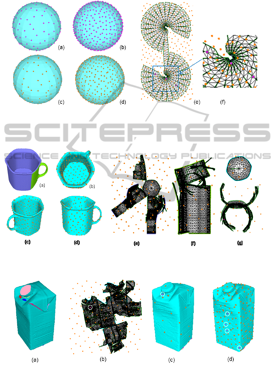
Figure 4: Sphere: #vertices =382; #edges=1140; #triangles=760; #strips=1; Hammersley algorithm in the spherical coor-
dinates: (a) #points=192, (b) #points=770; low-discrepancy points wrapping approach: (c) #points=192, R=1.32; (d)
#points=770, R=0.95; (e) 2D strip; (f) image enlargement.
Figure 5: Cup: #vertices =7024, #edges =20976, #triangles =13952, #strips=4; (a) segmentation; (b), (c) and (d) different
views of #points=550, R=0.30; (e), (f) and (g) 2D strips with #points=65 and R=1.73.
Figure 6: Fruit Drink: #vertices =12487, #edges =37495, #triangles =24994, #strips=32; (a) segmentation; (b) the largest
strip with 21963 triangles; (c) #points=56, R=1.07; (d) #points=315, R=0.22.
Low-DiscrepancyDistributionofPointsonArbitraryPolygonal3D-surfaces
85
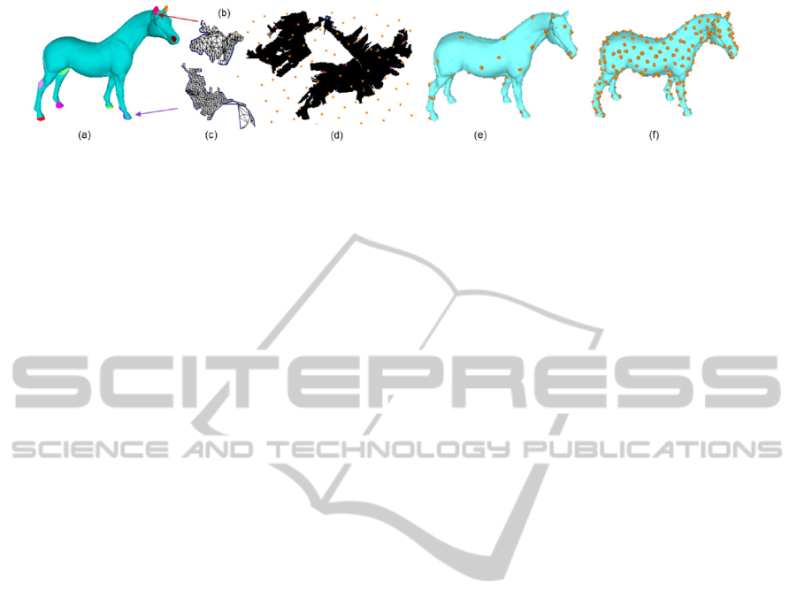
Figure 7: Horse: #vertices=48485, #edges=145449, #triangles=96966‚ #strips=28; (a) segmentation; (b) and (c) small 2D
strips with 252 and 520 triangles, respectively, (d) the largest 2D strips with 93754 triangles; (e) R=1.65, #points=57; (f)
R=0.25, #points=335.
ure 6b we also can see the pink points added by the
correction algorithm.
The last example in Figure 7 demonstrates the
application of our approach to a large model (see
http://www.cc.gatech.edu/projects/large_models/hor
se.html), whose mesh is produced by laser scanner
and has an unstructured grid, but it is well smoothed.
The mesh is cut into 28 segments. The mapping of
the largest one to the plane is shown in Figure 7d
and two smaller strips are given in Figure 7b and 7c.
The distribution of 335 points occurs with irregulari-
ty ratio R=0.25 and 28 sample points are scattered
with R=1.65.
6 CONCLUSIONS
In this work, we describe an approach for low-
discrepancy distribution of sample points on triangu-
lated surfaces of arbitrary 3D objects within a wide
density range. The accuracy of the performed tech-
nique is determined by the ratio between the area of
the irregular zone and the total area. A wide range of
possible point densities can be used to conform to
different level-of-details.
Our intent was to distribute as few points as pos-
sible on a 3D-surface so that from each view a suffi-
cient number of points is visible, which corresponds
to the visible fraction of the surface (with respect to
the required LoD). Examples indicate that good
results can already be achieved with less than 100
points, which is clearly smaller than the numbers
usually reported in literature (see Section 2).
An important question is how to perform the
segmentation and the unfolding in a way which
minimizes the raise in the discrepancy. The further
research will focus, therefore, on the mesh segmen-
tation and the unfolding as an optimisation problem.
Additional work will address the direct meas-
urement of the resulting geometric discrepancy on
the surface itself.
REFERENCES
Alexander, J. R., Beck, J, Chen, W. L., 2004. Geometric
discrepancy theory and uniform distribution. In Hand-
book of Discrete and Computational Geometry, Boca
Raton: Chapman & Hall/CRC, 2
nd
Edition.
Berg, M., 1996. Computing half-plane and strip discrep-
ancy of planar point sets. Comput. Geom. 6: 69-83.
Chen, W. W. L., Travaglini, G., 2007. Discrepancy with
respect to convex polygons. J. Complexity. 23(4-
6):662-672.
Cheng, J., Druzdzel, M. J., 2000. Computational investiga-
tion of low-discrepancy sequences in simulation algo-
rithms for Bayesian networks. In Proceedings of the
16th Conference on Uncertainty in Artificial Intelli-
gence. pp. 72–81.
Cui, J., Freeden, W., 1997. Equidistribution on the sphere.
SIAM J. Sci. Comput. 18(2):595–609.
Dachsbacher, C., Stamminger, M., 2006. Splatting indirect
illumination. In Proceedings of the 2006 symposium
on Interactive 3D graphics and games (I3D '06). pp.
93-100.
Grabner, P.J., Hellekalek, P., Liardet, P., 2012. The dy-
namical point of view of low-discrepancy sequences.
Uniform Distribution Theory. 7(1):11–70.
Halton, J. H., 1960. On the efficiency of certain quasi-
random sequences of points in evaluating multi-
dimensional integrals. Numer. Math.. 2:84–90.
Hammersley, J. M., 1960. Monte Carlo methods for solv-
ing multivariable problems. Ann. New York Acad. Sci..
86:844–874.
Hanson, K. M., 2003. Quasi-Monte Carlo: half-toning in
high dimensions?. In Proceedings SPIE 5016. pp.161-
172.
Hofer, R., Pirsic, G., 2011. An explicit construction of
finite-row digital (0,s)-sequences. Uniform Distribu-
tion Theory. 6:13–33.
Matousek, J, 1999. Geometric Discrepancy – An Illustrat-
ed Guide. Algorithms and combinatorics series,
Vol.18; Springer, Berlin Heidelberg.
Niederreiter, H., Chao, X, 1995. Low-discrepancy se-
quences obtained from algebraic function fields over
finite fields. Acta Arithmetica, 72:281–298.
Pillards, T., Cools, R., 2005. Transforming low-
discrepancy sequences from a cube to a simplex. J.
Comput. Appl. Math.. 174(1): 29–42.
GRAPP2014-InternationalConferenceonComputerGraphicsTheoryandApplications
86

Quinn, J. A., Langbein, F. C., Martin, R. R., 2007. Low-
discrepancy point sampling of meshes for rendering.
In: Symp. on Point-Based Graphics 2007. pp. 19-28.
Rakhmanov, E.A., Saff, E.B., Zhou, Y.M., 1994. Minimal
discrete energy on the sphere. Math. Res. Lett.. 1:647–
662.
Rovira, J., Wonka, P., Castro, F., Sbert, M., 2005. Point
sampling with uniformly distributed lines. Eu-
rographics Symp. Point-Based Graphics. pp. 109–118.
Shamir A., 2008. A Survey on Mesh Segmentation Tech-
niques. Computer Graphics Forum. 27( 6): 1539-
1556.
Sobol, I. M., 1967. On the distribution of points in a cube
and the approximate evaluation of integrals. U.S.S.R.
Computational Mathematics and Mathematical Phys-
ics, 7(4):86-112.
Wand, M., Straßer, W., 2003. Multi-resolution point-
sample raytracing. In: Graphics Interface 2003 Con-
ference Proceedings.
Wong, T.-T., Luk, W.-S., Heng, P.-A., 1997. Sampling
with Hammersley and Halton points. Journal of
Graphics Tools. 2(2):9-24.
Low-DiscrepancyDistributionofPointsonArbitraryPolygonal3D-surfaces
87
