Cardiovascular Dynamics during Head-up Tilt assessed Via a Pulsatile

and Non-pulsatile Model

N. Williams, H. T. Tran and M. S. Olufsen

Department of Mathematics, NC State University, Raleigh, NC, U.S.A.

Keywords:

Cardiovascular Dynamics Modeling, Head-up Tilt, Pulsatile vs. Non-pulsatile Modeling, Parameter Estima-

tion.

Abstract:

This study compares a pulsatile and a non-pulsatile model for prediction of head-up tilt dynamics for healthy

young adults. Many people suffering from dizziness or light-headedness are often exposed to the head-up

tilt test to explore potential deﬁcits within the autonomic control system, which is supposed to maintain the

cardiovascular system at homeostasis. However, this system is complex and difﬁcult to study in vivo. This

study shows how mathematical modeling can be used to extract features of the system that cannot be measured

experimentally. More speciﬁcally, we show that it is possible to develop a mathematical model that can predict

changes in cardiac contractility and vascular resistance, quantities that cannot be measured directly, but which

can be useful to assess the state of the system. The cardiovascular system is pulsatile, yet predicting control in

response to head-up tilt for the complete system is computationally challenging, and limits the applicability of

the model. In this study we show how to develop a simpler non- pulsatile model that can be interchanged with

the pulsatile model, which is signiﬁcantly easier to compute, yet it still is able to predict internal variables.

The models are validated using head-up tilt data from healthy young adults.

1 INTRODUCTION

Emergency rooms and syncope clinics see a large

number of people who have experienced lighthead-

edness or dizziness. These syndromes may be as-

sociated with orthostatic intolerance: the inability

to maintain blood pressure and ﬂow in response to

active standing or head-up tilt. Orthostatic intoler-

ance (Lanier et al., 2011) is triggered by a number

of factors, the most important being dysautonomia, a

disorder associated with the autonomic nervous sys-

tem.

In this study we use mathematical modeling to

predict blood pressure and heart rate dynamics ob-

served during HUT. The HUT protocol starts with a

subject resting in supine position on a tilt-table, after

steady oscillating values for heart rate and blood pres-

sure have been recorded, the subject is tilted head up

to a 60-70 degree angle. The test typically lasts be-

tween 10-20 minutes after initiation of the tilt. At this

point most subjects feel light-headed and are tilted

back to supine position. Upon tilting blood is pooled

in the lower body causing a drop in blood pressure

in the upper body, while blood pressure in the lower

body is increased. In response (for healthy subjects),

the autonomic system causes an increase in heart

rate, cardiac contractility, and peripheral resistance

redistributing blood volume and thereby reestablish-

ing homeostasis. For patients suffering from dysau-

tonomia, these responses may be partly or completely

inhibited.

More speciﬁcally, this paper compares a pulsatile

and a non-pulsatile mathematical model that can pre-

dict cardiovasculardynamics during HUT. Although a

pulsatile model for the cardiovascular system is bene-

ﬁcial, it enables analysis of dynamics within beats and

can be used to understand how modulation of the sys-

tem affects pulsatility (Williams et al., 2013), which

is useful in the study of the response immediately fol-

lowing HUT (within minutes of the tilt). However,

for numerous problems it is adequate to analyze the

system with the simpler non-pulsatile model. For ex-

ample, if the objective is to study dynamics associ-

ated with the entire procedure (10-20 min). In this

study we develop a non-pulsatile model for the car-

diovascular system that can predict HUT dynamics,

and show that parameters estimated with the non-

pulsatile model can be used within the pulsatile model

or possibly be combined with more complex models

including spatial information.

673

Williams N., T. Tran H. and S. Olufsen M..

Cardiovascular Dynamics during Head-up Tilt assessed Via a Pulsatile and Non-pulsatile Model.

DOI: 10.5220/0004624006730680

In Proceedings of the 3rd International Conference on Simulation and Modeling Methodologies, Technologies and Applications (BIOMED-2013), pages

673-680

ISBN: 978-989-8565-69-3

 2013 SCITEPRESS (Science and Technology Publications, Lda.)

Besides being able to interchange the non-

pulsatile and pulsatile models, in itself non-pulsatile

models have multiple advantages. First, since they

are less complex, coupling a non-pulsatile model with

more advanced models studying larger systems such

as the respiratory or renal systems becomes feasi-

ble. Moreover, with a simple model it becomes pos-

sible to study system dynamics over much longer

time-scales (hours-days). The respiratory cycle is

approximately a fourth of the cardiovascular cycle,

and control associated with respiratory dynamics take

min-hours (Hall, 2011). The renal system is one of

the most complex physiological feedback systems, it

interacts with the cardiovascular system, and feed-

back associated with this system is hours-days (Hall,

2011). Even if the objective is to study the impact of

fainting, often studied using HUT tests, it may be nec-

essary to use a simpler model. Typically, after HUT

it takes 10-20 minutes before the subject tilted ex-

periences light headedness (Lanier et al., 2011). Fi-

nally, it should be emphasized that computations with

the non-pulsatile are signiﬁcantly faster, in particu-

lar, since it is no longer necessary to account for the

discrete events associated with opening and closing

of the heart valves. In the following we will present

both a pulsatile and a non-pulsatile model and show

that they can be used interchangably in the study of

HUT dynamics.

2 METHODS

This section describes both the pulsatile and non-

pulsatile models, as well as the model changes im-

posed to predict gravitational pooling and autonomic

regulation necessary to predict HUT dynamics. We

ﬁrst describe the two models, we discuss HUT, and

methods needed for comparing model predictions.

2.1 Data

As a point of departure we use the model and model-

ing results presented in (Williams et al., 2013), which

develops and validates a pulsatile model predicting

HUT dynamics for ﬁve healthy young subjects. Since

our objective is to develop a non-pulsatile model us-

ing the same framework as the pulsatile model, we

modify the heart compartment, while the remaining

model compartments stay the same. To compare

the two models, we predict the moving average of

the pressures, cardiac output, and total blood volume

from the pulsatile model and compare results with

the non-pulsatile model. Comparisons are done using

sensitivity analysis, subset selection, and optimiza-

qvl

Cal

Vau

Cau

Up Body

Vvu

Cvu

pvu

Vlh

plh

Rvl

pau

Raup

RavRmv

qavqmv

Elh(t)

Left Heart

qaup

Ralp

qalp

Val

Vvl

ArteriesVeins

Lower Extremities

Upper Body

qal Ral

Low Body

pvl

pal

Cvl

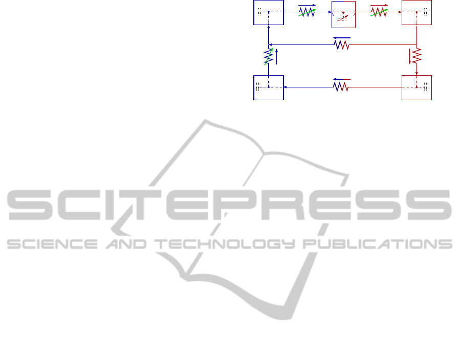
Figure 1: Compartment model predicting HUT dynam-

ics. For each compartment an associated blood pressure p

(mmHg), volumeV (ml), and compliance C (ml/mmHg) are

deﬁned. The compartments represent the upper body arter-

ies (subscript au), lower body arteries (subscript al), upper

body veins (subscript vu), lower body veins (subscript vl),

and the left heart (subscript lh). Resistances R (mmHg s/ml)

are placed between all compartments: R

denotes the resis-

tance between arteries in the upper and lower body, R

aup

and R

alp

denote resistance between arteries and veins in the

upper and lower body, respectively. For the pulsatile model,

the two heart valves, the mitral valve and the aortic valve,

are modeled as pressure dependent resistors R

and R

Finally, the resistance between the lower and upper body

veins R

is also modeled as pressure dependent to prevent

retrograde ﬂow into the lower-body during the HUT.

tion. More speciﬁcally, we estimate a set of model pa-

rameters minimizing the least squares error between

states computed by the two models. Only parameters

that represented differences between the two models

(i.e., the heart component) are allowed to vary.

2.2 Lumped Cardiovascular Models

This section describes the pulsatile and non-pulsatile

cardiovascular models depicted in Figure 1. These

models are developed to estimate blood ﬂow, volume,

and pressure in the systemic circulation during HUT

with and without a pulsating heart. Similar to the pul-

satile model (Williams et al., 2013), the non-pulsatile

model development is split into parts including devel-

opment of a lumped cardiovascular model estimating

dynamics while the subject is resting in supine posi-

tion; developing model components allowing predic-

tion of dynamic changes to HUT; and development of

methods for estimating the impact of cardiovascular

regulation on the model parameters.

Both models follow the same basic layout shown

in Figure 1, including four compartments represent-

ing arteries and veins in the upper and lower body

and a compartment representing the heart. The latter,

is the only compartment that differ between the two

models. Therefore, the general equations outlined be-

low are valid for both models.

For each compartment, a pressure-volume relation

SIMULTECH2013-3rdInternationalConferenceonSimulationandModelingMethodologies,Technologiesand

Applications

674

can be deﬁned as

−V

= C

− p

ext

), (1)

where V

(ml) is the compartment volume, V

(ml)

is the unstressed volume, C

(ml/mmHg) is the com-

partment compliance, p

(mmHg) is the compartment

instantaneous blood pressure, and p

ext

(mmHg) (as-

sumed constant) is the pressure in the surrounding tis-

sue. Moreover, for each compartment, the change in

volume is given by

= q

− q

out

, (2)

where q (ml/s) denotes the volumetric ﬂow. Using a

linear relationship analogous to Ohm’s law the vol-

umetric ﬂow q (ml/s) between compartments can be

computed as

q =

− p

out

, (3)

where p

and p

out

are the pressure on either side of

the resistor R (mmHg s/ml). Differentiating (1), using

(2), and inserting (3) allows us to obtain a system of

differential equations in blood pressure of the form



i−1

− p

i−1

−

− p

i+1



where i refer to the compartment for which the pres-

sure p

is computed, while i− 1 and i + 1 refer to the

two neighboring compartments. For resistances that

appear between compartments, R

i−1

refer to the resis-

tance between compartments i− 1 and i, and R

refer

to the resistance between compartments i and i + 1.

The latter equation is valid since we assume that C

(ml/mmHg) is constant. This formulation is utilized

for the four arterial and venous compartments.

For the pulsatile model, (2) describes the change

in volume of the left heart. Using a relation similar to

(1) we get

= E

−V

), (4)

where E

(mmHg/ml) is the left heart elastance (the

reciprocal of its compliance) and V

is the left heart

volume. Pumping is achieved by introducing a vari-

able elastance function (Ellwein, 2008) of the form

(

t) = (5)











−E

(1− cos(

) + E

t ≤ T

−E

(cos(

π(

t−T

)

) + 1) + E

t ≤ T

+ T

t ≤ T

where

t is the time within a cardiac cycle T = 1/H.

and E

denote the minimum and maximum elas-

tance, respectively. For each cardiac cycle elastance

is increased for 0 <

t < T

and decreased for T

t < T

+ T

, while during diastole T

+ T

t < T

elastance is kept constant at its minimum value. Val-

ues for T and T

are obtained from data, while T

a model parameter.

Finally, heart valves are modeled using pressure

dependent resistors for which a large resistance R

represents a closed valve, while a small resistance

represents an open valve. These are modeled as

smooth sigmoidal functions of the form

= R

−

− R

1+ e

−β(p

−p

out

)

, (6)

where p

and p

out

denote the pressures in compart-

ments on either side of the valve. For p

> p

out

→ R

(the valve is open), and when p

out

> p

→ R

(the valve closes).

The non-pulsatile heart model is adapted work

by Batzel et al. (Batzel et al., 2007), which fol-

lowed ideas originally proposed by Grodins (Grodins,

1959). This method does not explicitly model the

pumping of the heart, but predicts cardiac output Q

as a function of venous pressure p

. The original

model was used within a complete circulation. It pre-

dicted cardiac output as a function of pulmonary ve-

nous pressure, the current model only encompasses

the systemic circulation, consequently this study pre-

dicts cardiac output as a function of systemic venous

pressure p

The basic assumption concerning cardiac output,

i.e., the outﬂow of blood from the heart, for non-

pulsatile ﬂow states that: Given the heart rate H (in

strokes per minute) the ﬂow of the left ventricle Q

generated by a ventricle is given by

Q = HV

str

, (7)

where V

str

is the stroke volume, i.e., the volume of

blood ejected during one stroke. As a result time vary-

ing quantities in the non-pusatile model are to be in-

terpreted as averages over the length of a pulse. The

stroke volume is given by

str

= V

−V

, (8)

where V

is the end-diastolic volume and V

is the

end-systolic volume of the heart.

Another assumption involves expressing stroke

volume V

str

as a function of the arterial and ve-

nous pressures acting on the ventricle. Concerning

the ejection phase of the heart cycle we have the

so called Frank-Starling mechanism (Burton, 1972),

which states that the stroke volume of the heart in-

creases in response to an increase in the volume of

blood ﬁlling the heart (the end diastolic volume) when

all other factors remain constant. Consequently, in-

creased ﬁlling of the ventricle during diastole, causes

an increased contraction force during the following

CardiovascularDynamicsduringHead-upTiltassessedViaaPulsatileandNon-pulsatileModel

675

systole.

str

−Vun), (9)

where p

is the arterial pressure against which the

ventricle has to eject (the afterload) and S denotes the

contractility of the left ventricle.

Using the previous two assumptions we express

the ventricular output Q (the cardiac output) as a func-

tion of blood pressure. To model the ﬁlling process of

the heart, when the mitral valve is open, we assume

that the inﬂow in to the ventricle depend on the differ-

ence between the ﬁlling pressure and the left ventricle

pressure, using an expression analogous to (3), we get

(t) =

− p

), (10)

where V

is the ventricular volume at time t after the

ﬁlling process has started, p

is the ventricular pres-

sure, p

is the venous ﬁlling pressure assumed to be

constant, and R

is the total ventricular resistance to

the inﬂow of blood.

For the relaxed ventricle, a similar volume-

pressure relation can be derived (e.g., as in (1)),

V(t) = C

(t) +V

, (11)

where V

denotes the unstressed volume of the re-

laxed ventricle and C

denotes the heart compliance.

The initial value for (10) is given by V(0) = V

. Us-

ing (11) in (10), integrating, and letting t = t

, the

time of end-diastole, we obtain

= kV

+ a(C

), (12)

where k = exp(−t

) and a = 1− k.

Equations (8), (9), and (12) constitute a system of

linear equations for V

, V

, and V

str

. We obtain

= C

−

+ kS

, (13)

= C

−

+ kS

, (14)

str

+ kS

. (15)

Combining (7) and (15) gives the cardiac output

out of the ventricle

Q = H

+ kS

, (16)

where H is heart rate,C

heart compliance, p

venous

pressure, p

arterial pressure, and S contractility.

There are essentially two possibilities for a ventri-

cle to change the cardiac output: to change the heart

rate or the contractility. Heart rate and contractility

are related through the Bowditch effect (Klabunde,

1972), which states that contractility is proportional

to heart rate. The Bowditch effect can be accounted

for by introducing the second order ordinary differen-

tial equation, of the form

S+ γ

S+ αS = βH, (17)

where γ, α, and β are positive constants and H is heart

rate. For this study, we rewrite this second order ODE

as two ﬁrst order equations.

Using these relations the pulsatile ﬁve differential

equations can be written as

= (q

− q

aup

)/C



− q

alp





alp

− q



= (q

aup

+ q

− q

)/C

= q

− q

and the non-pulsatile equations as

= (Q− q

− q

aup

)/C



− q

alp





alp

− q



= (q

aup

+ q

− Q)/C

= σ

dσ

= −αS− γσ+ βH,

where

− p

aup

− p

aup

− p

alp

− p

alp

− p

In the last set of equations the left ventricular pressure

) is predicted using (4), the pressure dependent re-

sistances used to model the valves (R

) are pre-

dicted from (6), and the total blood volume can be

SIMULTECH2013-3rdInternationalConferenceonSimulationandModelingMethodologies,Technologiesand

Applications

676

computed from pressures using (1). These equations

were solved in Matlab using the ODE15s differential

equations solver. Abbreviations (subscripts) are given

in Table 1.

2.2.1 Modeling HUT

As the subject is tilted (shown in Figure 2), blood is

pooled in the lower extremities leading to an increase

in pressure in the lower body, while pressure in the

upper body decreases. To account for gravity, the

pressure at the level of the carotid arteries are used

as a reference pressure, so an extra term is added to

the ﬂow (q

) and subtracted from the ﬂow (q

) of the

lower body compartments. The gravitational effects

are calculated as described by Olufsen et al. (Olufsen

et al., 2005; Williams et al., 2013), giving the follow-

ing modiﬁed ﬂow equations

q =

ρgh

tilt

sin(θ(t)) + p

− p

out

, (18)

θ(t) =

180







0 t < t

(t − t

) t

≤ t ≤ t

+ t

60 t > t

+ t

where ρ (g/ml) is blood density, g (cm/s

) is the con-

stant of gravitational acceleration, h

tilt

(cm) is the

absolute height between the upper body and lower

body compartments, θ(t) is the tilt angle (in radians),

= 15 degrees/s is the tilt speed, while t

and t

denote the time at which HUT is started and ended,

respectively. The combined term ρgh

tilt

sin(θ(t)) de-

notes the hydrostatic pressure between the upper and

lower body compartments.

2.2.2 Modeling Effects of Cardiovascular

Regulation

Upon HUT ﬁring of the baroreceptor nerves are mod-

ulated by the aortic and carotid sinus baroreceptors

sensing changes in the stretch of the arterial wall.

Typically, HUT leads to a decrease in blood pressure

mediating an increase in sympathetic outﬂow along

Table 1: Abbreviations (subscripts) used in the compart-

mental model.

Abbreviation Name

av aortic valve

au upper body arteries

al lower body arteries

aup upper body ”peripheral” vascular bed

alp lower body ”peripheral” vascular bed

vu upper body veins

vl lower body veins

lh the left heart (ventricle and atrium)

Figure 2: The HUT test: The subject depicted is tilted to

an angle of 60 degrees at a constant speed of 15 degrees

per second. Red and yellow circles indicate the locations

for the blood pressure sensors. Each sensor is mounted on

the index ﬁnger, one ﬁnger (red) is placed at the level of

the carotid artery, while the other (yellow) is placed at the

level of the heart. Upon HUT blood is pooled in the lower

extremities.

with parasympathetic withdrawal. Sympathetic stim-

ulation elicits changes in vascular resistance and car-

diac contractility, while parasympathetic withdrawal

primarily has an effect on heart rate and cardiac con-

tractility. Heart rate is used as an input, consequently,

parasympathetic heart rate regulation is implicitly ac-

counted for in the model. For the pulsatile model,

regulation of cardiac contractility is modeled by con-

trolling the minimum elastance of the left heart (E

)

and vascular resistance is regulated in both the up-

per and lower body. However, as the compartments

representing the upper and lower body arteries appear

in parallel, both resistances are not identiﬁable. We

controlled R

aup

directly, while we let R

alp

= kR

aup

where k is the ratio of the optimized supine values of

aup

and R

alp

. For the non-pulsatile model, we do not

have an explicit expression for E

, instead contrac-

tility is included via the Bowditch effect (Klabunde,

1972), and modeled as a function of heart rate as de-

scribed in (17). Hence, changes in contractility has

been modeled indirectly, via the 2’nd order ODE,

while parameters associated with autonomic control

of vascular resistance should be modeled. To so, sim-

ilar to (Williams et al., 2013) we predict R

aup

as a

piece-wise linear function given by

X(t) =

∑

i=1

K(t), (19)

K(t) =











t − t

i−1

− t

i−1

, t

i−1

≤ t ≤ t

i+1

− t

i+1

− t

≤ t ≤ t

i+1

0, otherwise

where the unknown coefﬁcients γ

, i = 1...N are the

new parameters that will be estimated to predict the

CardiovascularDynamicsduringHead-upTiltassessedViaaPulsatileandNon-pulsatileModel

677

control. N is the number of nodes along the time span

analyzed. The spread of the N nodes should be spec-

iﬁed in the model. For simulations reﬂecting dynam-

ics observed in supine position we placed the nodes

with a frequency of 6-10 seconds, but during HUT,

where dynamics change, signiﬁcantly more points are

added. It should be noted that the more points are

added to the time-span, the longer the simulations.

3 RESULTS

We ﬁrst show results obtained for a subject in supine

position followed by results obtained when the same

subject is tilted upright to a 60 degree angle (see Fig-

ure 2). Results during supine position are included to

tune model parameters to the subject studied, while

during HUT we allow parameters regulated by the

autonomic control system to vary in time. For each

event we estimate parameters minimizing the least

squares error between the model output and data. To

develop two models (pulsatile and non-pulsatile) that

can be interchanged, we compute moving averages

for the quantities X = {p

, p

, CO

, V

tot

}

using pulsatile model outputs predicted in Williams

et al. (Williams et al., 2013), and use these as data for

the non-pulsatile model.

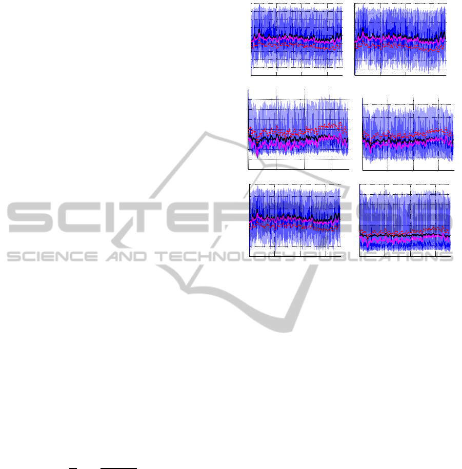
3.1 Optimization During Supine

Position

First we predict dynamics during supine position, as

stated above. These simulations are included to tune

the model to the subject studied. For these simu-

lations we estimate parameters in the non-pulsatile

heart model (R

, C

, α, β, γ, c) minimizing the least

squares error

J =

∑

i=1



− X



where X denotes the states listed above, super-

script d refers to the data (obtained from the pul-

satile model (Williams et al., 2013)), and superscript

m refers to results obtained with the non-pulsatile

model.

It should be noted that parameters ”not” associ-

ated with the heart compartment are kept constant,

since they represent components common for the two

models. Results comparing the pulsatile and non-

pulsatile model during steady state are shown in Fig-

ure 3. This ﬁgure shows all pressures and cardiac

output. Each graph shows pulsatile model results

(from Williams et al. (Williams et al., 2013)), moving

0 50 100 150

pau (mmHg)

0 50 100 150

pal (mmHg

0 50 100 150

2.6

2.7

2.8

2.9

3.1

3.2

3.3

pvl (mmHg)

0 50 100 150

2.2

2.4

2.6

2.8

3.2

pvu (mmHg)

0 50 100 150

100

110

120

time (s)

CO (ml/s)

0 50 100 150

4400

4600

4800

5000

5200

5400

5600

5800

time (s)

Vtot (ml)

Figure 3: Predictions during supine position. All graphs in-

clude the pulsatile model output (blue), the mean of the pul-

satile model output (black), the non-optimized (red, dashed)

and optimized (magenta) non-pulsatile model output for the

upper and lower body arterial pressure p

and p

, upper

and lower body venous pressure p

and p

, cardiac output

CO, and total volume V

tot

averages predicted from the pulsatile model (black

line), computations with the non-pulsatile model us-

ing nominal parameters (red dashed line), and com-

putations with optimized parameters for the non-

pulsatile model (magenta line). Note that for all states

the two models agree well.

Initial parameters used for the arterial and venous

portions of the model (results not shown) were esti-

mated as described in previous studies Williams et

al. (Williams et al., 2013). In short, we used sen-

sitivity analysis and subset selection to obtain a set

of parameters that can be estimated given the model

and available data, and used nonlinear optimization

to estimate their value. For this study, we only es-

timated parameters associated with the heart com-

ponent within the non-pulsatile heart, assuming the

tuned arterial and venous parameters found within the

pulsatile model can be used within both formulations.

3.2 HUT Optimization

Once baseline parameters were obtained, we imposed

HUT, by modifying ﬂows between the upper and

lower body as described in (18). For these simula-

SIMULTECH2013-3rdInternationalConferenceonSimulationandModelingMethodologies,Technologiesand

Applications

678

tions, we only estimate the control parameters θ =

Raup,i

used for computing R

aup

as stated in (19), i.e.,

we let the parameter R

sup

vary in time. In the pul-

satile model we also let contractility be time-varying,

via estimation of γ

Em,i

, yet the non-pulsatile model

directly accounts for this part of the control via the

Bowditch effect (17), predicting cardiac contractility

S as a function of heart rate H. For this portion of

the model, we only included p

in the cost function,

giving

J =

∑

i=1

au,i

− p

au,i

where superscript d refers to the data and superscript

m for the model.

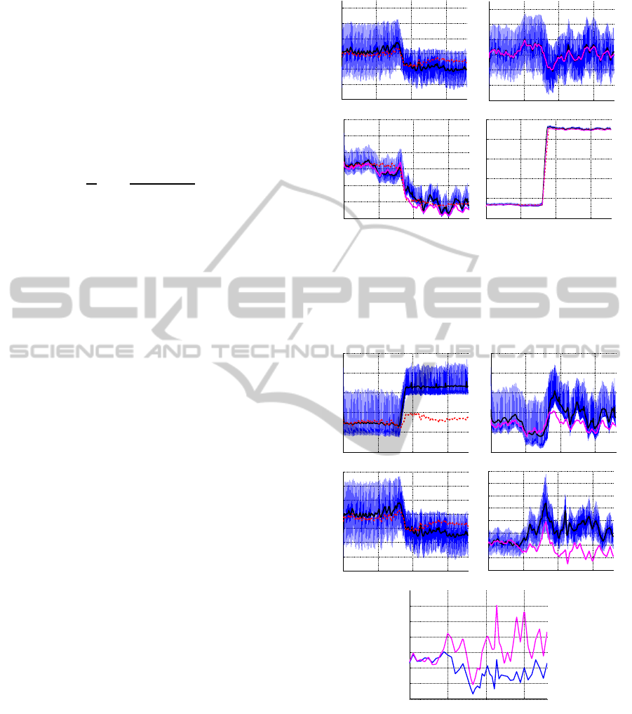
Figure 4 shows the pulsatile model output (blue),

the moving average data computed from the pulsatile

model (black), and results using nominal parameter

values (red dashed) during HUT. The subject is tilted

after 80 sec and remains upright for the duration of

the simulation. The top left graph in Figure 4 de-

picts dynamics without activating the control, i.e., for

this simulation R

aup

is kept at its baseline value. Note

that after about 100 sec, this part of the model devi-

ates slightly from results obtained with the pulsatile

model. This is likely due to the fact that the non-

pulsatile model results already incorporate control of

contractility (S), while the ”data” obtained from the

pulsatile model were obtained using constant contrac-

tility values E

. The following graphs show all model

predicted pressures obtained with the non-pulsatile

model using optimal parameter values. Note that pre-

dictions for p

are signiﬁcantly closer than for the

other states, this is likely because for these simula-

tions, we only include p

in the cost function. In

other words, no effort was made to account for varia-

tion in the remaining states. Finally, Figure 5 shows

corresponding volumes and cardiac output, both are

shown with nominal and optimized parameter values.

This ﬁgure also shows time-varying prediction of pe-

ripheral vascular resistance R

sup

The signiﬁcance of the relation between the pul-

satile and non-pulsatile models are corroborated fur-

ther by examining dynamics of quantities for which

data are not available, i.e., for p

, p

, and p

de-

picted in Figure 4. Finally, our model provides good

predictions of blood volume and cardiac output, de-

picted for a representative subject in Figure 5.

4 CONCLUSIONS

This study has shown that it is possible to develop

a pulsatile and a non-pulsatile model that can both

0 50 100 150

100

pau (mmHg)

time (s)

0 50 100 150

100

pau (mmHg)

0 50 100 150

1.5

2.5

3.5

pvu (mmHg)

0 50 100 150

pvl (mmHg)

Figure 4: Predictions during HUT. Pulsatile (blue), mov-

ing average from pulsatile model (magenta), non-pulsatile

model with nominal (red dashed) and optimized (magenta)

parameter values. The top graph shows p

predicted using

nominal parameter values. The following four panels com-

pares arterial and venous pressures in the upper and lower

body.

0 50 100 150

4000

4500

5000

5500

6000

6500

Vtot (ml)

0 50 100 150

4000

4500

5000

5500

6000

6500

Vtot (ml)

0 50 100 150

100

110

120

CO (ml/s)

0 50 100 150

100

120

140

160

180

200

time (s)

CO (ml/s)

0 50 100 150

0.4

0.6

0.8

1.2

1.4

1.6

time (s)

Raup (mmHg s/ml)

Figure 5: Volume and CO predictions during HUT. The top

two graphs depict the total blood volume during HUT with-

out (left) and with (right) cardiovascular regulation. The

following two graphs show cardiac output computed with-

out (left) and with (right) cardiovascular regulation. Again,

pulsatile (blue), pulsatile mean values (black), and non-

pulsatile (red, dashed) denote simulations with nominal and

(magenta) with estimated parameter values. The bottom

graph shows estimated values for R

aup

with pulsatile (ma-

genta) and non- pulsatile (blue) models.

CardiovascularDynamicsduringHead-upTiltassessedViaaPulsatileandNon-pulsatileModel

679

predict dynamics during HUT, and that time-varying

parameters (R

aup

) can be predicted by both models.

Moreover, we have shown (graph not included) that it

is possible to use parameter estimates obtained with

the non-pulsatile model within the pulsatile model.

This could be used in simulations done over long

time-scales (min-hours) where it may only be neces-

sary to study pulsatility intermittently, e.g., following

given events within the system. Finally, it should be

noted that compartments and parameters associated

with the arterial and venous subsystems are identical

for the two models. The only difference is the com-

partment predicting dynamics of the left heart.

In summary, we have developed a non-pulsatile

model and shown that it can be used to predict HUT

dynamics. These models (the pulsatile and non-

pulsatile models) have many potential beneﬁts for the

study of complex models, which contain a cardiovas-

cular component. The advantage of results presented

here is that the non-pulsatile model has potential to

be included in for applications that require analysis of

data over large time-scales.

ACKNOWLEDGEMENTS

Williams and Olufsen were supported in part by

the virtual rat physiology project (VPR) supported

by NIH-NIGMS under grant #1P50GM094503-01A0

sub-award to NCSU. Tran and Olufsen were also sup-

ported by NSF under the grant NSF/DMS #1022688.

REFERENCES

Batzel, J., Kappel, F., Schneditz, D., and Tran, H. (2007).

Cardiovascular and respiratory systems: modeling,

analysis, and control. SIAM, Philadelphia, PA.

Burton, A. (1972). Physiology and biophysics of the cir-

culation: an introductory text. Year Book Medical

Publishers Inc, Chicago, IL.

Ellwein, L. (2008). Cardiovascular and respiratory mod-

eling. PhD thesis, Department of Mathematics, NC

State University, Raleigh, NC.

Grodins, F. (1959). Integrative cardiovascular physiology:

a mathematical synthesis of cardiac and blood vessel

hemodynamics. Q Rev Biol, 34:93–116.

Hall, J. (2011). Guyton and Hall Textbook of Medical Phys-

iology. Saunders, Philadelphia, PA, 12th edition.

Klabunde, R. (1972). Physiology and biophysics of the cir-

culation: an introductory text. Lippincott Williams

and Wilkins, Philadelphia, PA.

Lanier, J., Mote, M., and Clay, E. (2011). Evaluation

and management of orthostatic hypotension. Am Fam

Physician, 84:527–536.

Olufsen, M., Ottesen, J., Tran, H., Ellwein, L., Lipsitz, L.,

and Novak, V. (2005). Blood pressure and blood ﬂow

variation during postural change from sitting to stand-

ing: model development and validation. J Appl Phys-

iol, 99:1523–1537.

Williams, N., Wind-Willassen, O., Program, R., Mehlsen,

J., Ottesen, J., and Olufsen, M. (2013). Patient speciﬁc

modeling of head-up tilt. Math Med Biol, In press.

SIMULTECH2013-3rdInternationalConferenceonSimulationandModelingMethodologies,Technologiesand

Applications

680