
Slope based Grid Creation using Interpolation of LIDAR Data Sets
Jan Hovad, Jitka Komarkova and Pavel Sedlak
Faculty of Economics and Administration, University of Pardubice, Studentska 84, 532 10 Pardubice, Czech Republic
Keywords: DTM, LIDAR, Interpolation, Grid, Surface.
Abstract: This article proposes a new approach of DTM creation from irregular LIDAR data scan. It shows the new
way how to utilize GIS results in the 3D modelling branch. LIDAR has a form of digital model of relief
which does not include artificial objects on the surface. DEM is created on the basis of individual points and
their elevation values and is further used for segmentation and classification of the terrain. Key attribute for
this operation is computation of the slope in the area of interest. Resulting classes are used as vector
outlines. These outlines are intended to divide the point cloud into groups. Each of them has specific
requirements for resolution. Flat areas can be modelled with less detail whilst hilly regions with sharp
elevation changes require higher resolution. LIDAR input is processed by chosen interpolation method, in
this case IDW and Renka-Cline algorithm. Irregular structure of the point cloud is converted into regular
grid of points. This process is semi-automatic. It is implemented in C++ library in the application Origin.
Output is automatically saved in predefined variable resolution (set of grids) and prepared to be processed in
3D.
1 INTRODUCTION
Light detection and ranging (LIDAR) is technology
that provides information about elevation of scanned
objects and their position. This technology is utilized
in this article. Goal of this study is based on the
previous research of authors. In this case, authors
were looking for a method that could eliminate the
disadvantages of triangulated irregular networks
(TINs) and that lowers the hardware requirements as
much as possible (Axelsson, 2000).
Current applied utilization of LIDAR is very rich
and intersects a wide range of scientific disciplines.
Most frequent example is creation of Digital Terrain
Model (DTM). Practical example of the DTM
creation can be found in research from Mandlburger
et al. (2009) who studied hybrid terrain models in
the river flow modelling. Next one is the Digital
Elevation Model (DEM). It is frequently used to
compute elevation based analyses. The Digital
Height Canopy Model (DHCM) is used for
reconstruction of forests and vegetation. This
research was done by Klimanek (2006) who used
LIDAR technology in the forestry.
Reconstructed model of terrain relief can be
enriched by buildings in the form of the Digital
Building Model (DBM) and can be used for example
for antennae signal prediction or navigation (Li et al.
(2007). All of these parts can be merged together to
form one complex model. Prerequisite for this
operation is data processing described in this text.
2 IDENTIFIED ISSUES
AND GOALS IN GRID
CREATION
The main goal of this paper is to create slope based
set of quadrilateral grids. This grid set can be made
by chosen interpolation method which can compute
unknown value at a specific grid from the known,
measured values. It is usually represented with
certain error. Interpolated outputs can be stored as a
set of LIDAR XYZ files. These files can be further
processed by 3D applications in parametrical and
procedural way to form almost photo-realistic
visualisation with maintaining the presence of GIS
analyses.
Partial steps can be summarized as follows: (1)
Batch operations are handled by basic scripting and
programming (C++) (2) Resulting grids have a form
of quadrilaterals and they are saved as XYZ files in
the form that will be handled by any 3D scripting
227
Hovad J., Komarkova J. and Sedlak P..
Slope based Grid Creation using Interpolation of LIDAR Data Sets.
DOI: 10.5220/0004574402270232
In Proceedings of the 8th International Joint Conference on Software Technologies (ICSOFT-EA-2013), pages 227-232
ISBN: 978-989-8565-68-6
Copyright
c
2013 SCITEPRESS (Science and Technology Publications, Lda.)
language in next research. (3)This processed grid
can be used further for visualization, simulation or it
can be utilized in any other scientific field, previous
steps are prerequisites for this operation (4)
Demonstration in the large area in the form of terrain
model by use of constant grid.
2.1 Inputs and Outputs of Individual
Operations
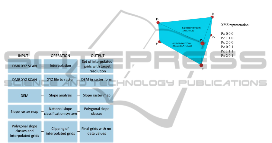
Outline of all key operations to reach set goals can
be expressed by a simplified scheme of inputs and
outputs (Figure 1). This expression represents the
chained pipeline. The first input (LIDAR irregular
data set) is processed through the entire process
while partial output files are generated and re-used
in the next steps.
Figure 1: Processing scheme.
2.2 Used Data and Software
This chapter describes the used data and software
that was needed to finish set goals. Authors had
mainly one available input to finish them. LIDAR
scan for area size 10×20 km. Source of data is from
the Military Office for Geography and
Hydrometeorology of Army of the Czech Republic.
Data set is scanned by aircraft Turbolet L-410 FG.
Scanning parameters are set to, fly height = 1200 m,
plane speed = 250 km/h, beam frequency = 80-120
kHz, scan angle = 60°, scan direction = East-West,
width and length of scanned stripe = 0,8 - 25/60 km
and sides are overlapped by 50 %. Outputs resulted
in two types of LIDAR models. First, the Digital
Surface Model 1st generation (DSM 1G) which
included all objects on the surface (terrain +
vegetation, buildings,…). Second, the Digital Model
of Relief 5
th
generation (DMR 5G). For this purpose
is the DMR sufficient because authors solved only
problems directly connected with terrain (Belka,
2012).
Scanned data are stored as XYZ text files. Each
scanned point is represented by separate line with
information about X/Y coordinate (WGS 1984) and
Z elevation attribute (meters above sea level). Area
is scanned and saved separately into 50 files that
formed a rectangular matrix. These individual files
are merged together and formed 800 MB big file that
consisted 21 000 000 records (points). XYZ object
representation is plain and can be demonstrated by
basic object primitives (Figure 2).
Figure 2: XYZ file object representation.
This simplicity is from other side compensated by
hardware requirements. Authors used two computers
to perform individual operations. AMD Opteron and
Intel i7 2600K CPU, with minimum of 16 GB
memory, fast SATA III SSD (500 MB/s) and
GeForce 460 GTX. The most important is high
amount of memory to work with a large number of
points. This fact is reflected in the used software that
is mainly used as 64 bit versions to fully utilize
RAM capacity. The first one is ArcGIS 10 from
ESRI - this application fully sufficed in all
interpolation tasks based on local IDW algorithm
and also prepared the LIDAR data set. Batch tasks in
ArcGIS are made with the help of scripting language
Python. The second suitable application is
OriginLab. This application supports scripting,
utilizes national algorithm library (NAG) and
connects all the features within C++.
3 SIMPLIFYING LIDAR DATA
SET BY INTERPOLATION
This chapter characterizes the basic principle of
interpolation in case of simplifying irregular LIDAR
scan to regular grid structure.
3.1 LIDAR Interpolation
Interpolation is the estimation of attribute (in this
case elevation-Z) at unmeasured-unknown points
ICSOFT2013-8thInternationalJointConferenceonSoftwareTechnologies
228
from measured points (known points). Weather
forecast is a typical example of interpolation used in
real life. Temperatures are measured at
meteorological stations (known values) and
interpolated throughout the whole area of interest.
Points outside of it can be extrapolated. DEM is
often created from contour lines. To create
continuous raster surface, attributes (Z) from the
contour polyline must be interpolated into the
required grid with predefined unit resolution.
This is called the 2D interpolation because the
values are interpolated on the surface that is defined
by X and Y coordinates. It must be taken on mind
that even contour lines are frequently already based
on interpolation. In addition to these core
applications there are other input data types that can
be chosen for interpolation (points, lines, areas).
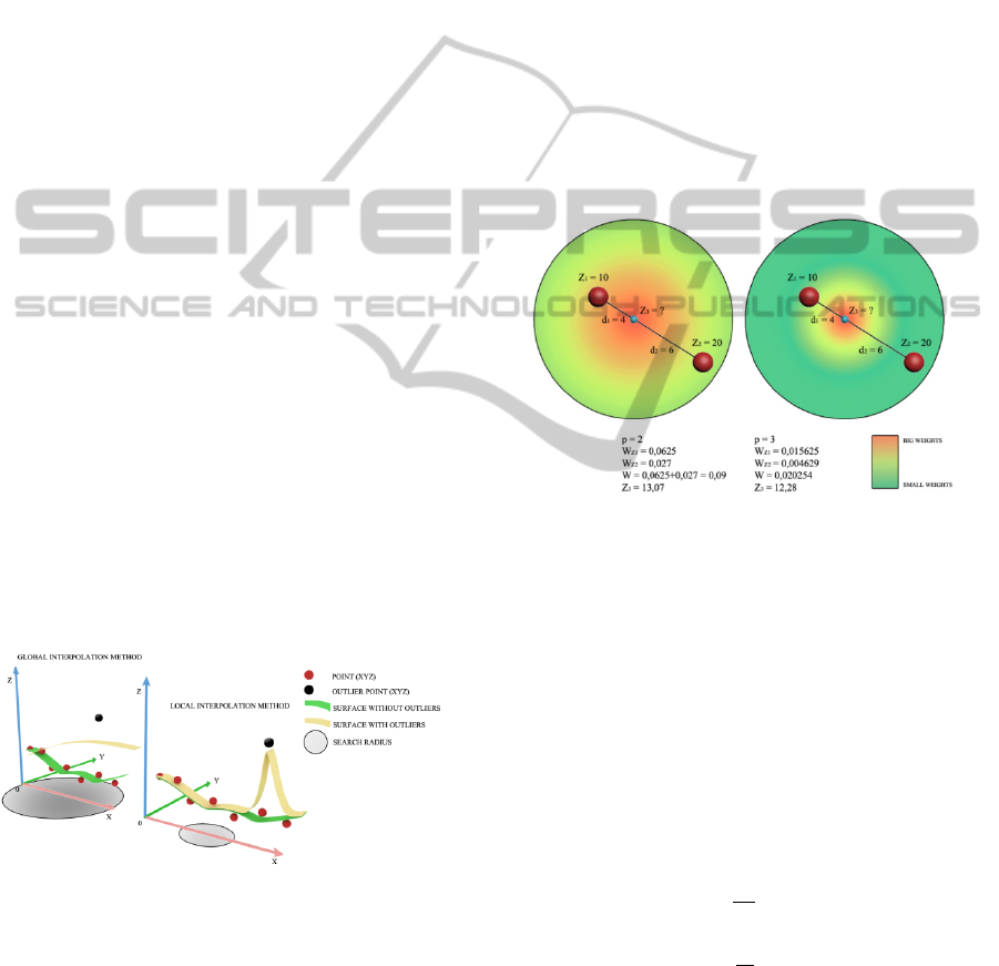
Interpolation process can be divided in two main
groups. Global interpolation considers all known
points and computes the unknown values at
specified location. Local interpolation method
usually sets the distance radius (variable or fixed)
around the known point and searches within it
throughout the limited number of neighbourhood
points for the computed value at specified position.
The difference between them is the sensitivity to an
outlier values.
This problem points to the fact that global
method creates smooth surfaces and local method
less smooth surfaces. Local method is not so
sensitive to outliers but creates spikes. This issue
must be considered before using available LIDAR
data set which can be noisy and uncorrected from
outlier values that were reflected from the unwanted
objects (Figure 3).
Figure 3: Global and Local interpolation methods.
Global interpolation can be represented by a surface
which is calculated with a polynom of specified
polynomial grade. For example linear (first grade),
quadratic (second grade), cubic (third). Higher grade
of polynom causes better curve/plane fitting through
the points. But from another aspect it cases so called
“Runges phenomenon” which computes wrong
estimations of attributes for unknown points (peaks).
The most used local interpolator which is used
also in this text is Inverse Distance Weighted
Average (IDW). This method is based on the
weighting the known attributes by an inverse power
of distance between known and unknown point. The
closer the unknown point is to a known point, the
stronger the influence of the distance.
User can specify parameters which affect the
output. p = exponent, 0 = no matter where the
unknown point is, 1 = direct correlation with the
distance, 2 = inverse power correlation with
distance, 3 and more = higher influence of
neighbourhood known points on the unknown points
computation. Radius and number of known points
used for computation - spatially affects the output.
All these parameters must be carefully checked
based on distribution of known data points (Figure
4) (Longley et al., 2011).
Figure 4: IDW power influence.
3.2 Batch Implementation
This text uses local interpolation of IDW and global
version of Renka-Cline interpolation (Renka and
Cline, 1984). IDW is computed in ArcGIS 10. Raw
LIDAR data are loaded as 3D features. XY
coordinates are additionally attached and the whole
irregular structure is batch processed by a Python
script. Script saves all interpolated grid outputs into
specified folder. Each output is saved in different
resolution defined by a target size of required
polygon.
(1)
(2)
Where, i = item in the array of resolutions, C
Xi
=
number of columns (X axis), R
Yi
= number of rows
(Y axis), W = width of the area of interest, H =
height of the area of interest, P
i
= target size of the
polygon.
SlopebasedGridCreationusingInterpolationofLIDARDataSets
229
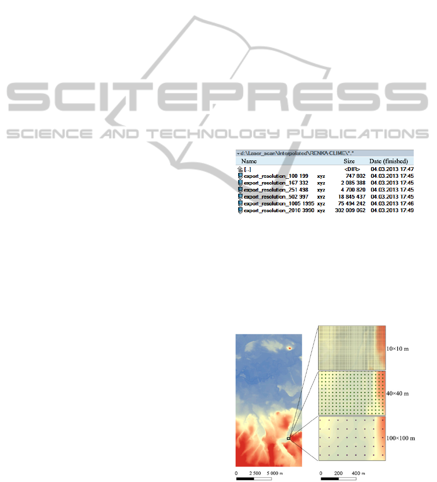
The whole area of interest has a size of 10×20
km. Target size of polygons is set to array of {5 10
20 40 60 100} meters. Computation resulted in two
input arrays, COLS {100,167,251,502,1005,2010},
ROWS {199,332,498,997,1995,3990}. Besides
Python script in ArcGIS, authors use application
OriginLab which combines scripting and
programming steps to fully customize the
computational process.
OriginLab uses C++ compiler and a NAG library
(Numerical Algorithm Group) which contains
approx. 1600 mathematical and statistical
algorithms. Following C++ code shows the batch
solution of performing Renka-Cline within an
application OriginLab. Source code shows only
basic procedure and script text output due to the
limits of article size. User specifies the input file
with LIDAR scan. In this case it is 800 MB big XYZ
data set. Active layer is loaded into XYZFile object.
XFBase class provides an access to scripting
functions, in this study xyz_renka from NAG
library. After that, data are iteratively processed and
saved separately. Timer shows the length of the
computational process and saving operations. Saving
a large xyz file can take a significant amount of
time. In case of grid resolution = 2010×3990 (8
million of points) over 2 minutes and iteration
generated 300 MB big grid file. Files are stored in
created directory.
void renka()
{
Alg = "RENKA-CLIME";
open_file();
Worksheet XYZFile =
Project.ActiveLayer();
for (int i=0;i<max;i++)
{
timerStart = GetTickCount();
int_to_fixed_str(gridValuesX[i],3,bufX)
int_to_fixed_str(gridValuesY[i],3,bufY)
outRes = bufX +" "+ bufY;
XFBase xf("xyz_renka_nag");
data.Add(XYZFile, 0, "X");
data.Add(XYZFile, 1, "Y");
data.Add(XYZFile, 2, "Z");
xf.SetArg("iz",data);
xf.SetArg("rows",gridValuesX[i]);
xf.SetArg("cols",gridValuesY[i]);
xf.Evaluate();
timerEnd = GetTickCount();
line;
printf("Algorithm: Renka-Clime\n");
printf("Resolution:%d",gridValuesX[i],"
× ",gridValuesY[i]);
printf("\nValues:%d\n",gridValuesX[i]*g
ridValuesY[i]);
printf("Pure computation completed
in:%d ms\n",timerEnd-timerStart);
convertMatrix();
Export_ASCII();
timerEndSave = GetTickCount();
printf("Saving the output file took :
%d ms\n",timerEndSave-timerEnd);
printf("Total time: %d
ms\n",timerEndSave-timerStart);
line;
}
printf("\n");
}
***************************
Algorithm: Renka-Clime
Resolution: 2010
Values: 8019900
Pure computation completed in : 11544
ms
Saving the output file took : 3370 ms
Total time: 14914 ms
***************************
Following figure shows the data output of
interpolation process. Set of grids are characterized
by an ascending resolution (Figure 5).
Figure 5: Data output of interpolation process.
The same situation applies to IDW grid set which is
created in ArcGIS. Grid can be stored either as a
point feature or a raster image. Figure 6 shows three
of six created grids in both forms, as raster and point
features. The big sized image on the left is the whole
area of interest. Black square outline magnifies the
area to show the finest details in the grid resolution.
Figure 6: Interpolated grids as raster and point features.
ICSOFT2013-8thInternationalJointConferenceonSoftwareTechnologies
230
4 GRID SEGMENTATION USING
DEM SLOPE ANALYSIS
This part is focused on the creation of clip polygons
in ArcGIS. These polygons will be used to clip the
computed set of XYZ grids which resulted from the
interpolation process. In this example authors used
three types of grids. Grid 1 has cell size of 5 meters,
suitable for hilly regions with sudden elevation
changes. Then Grid 2 has the cell size of 20 meters,
for highlands. The Grid 3 has the cell size of 60
meters, for flat lands. Reason for excluding other
grids is based in grid comparison. This comparison
is made by computing grid volumes and split sample
validation. Detailed results of these tests go beyond
of the subject of this article. They will be explained
further in next research. This fragmentation provides
the ability to process large territory. It would not be
possible with constant grid of 5×5 meters because of
hardware requirements.
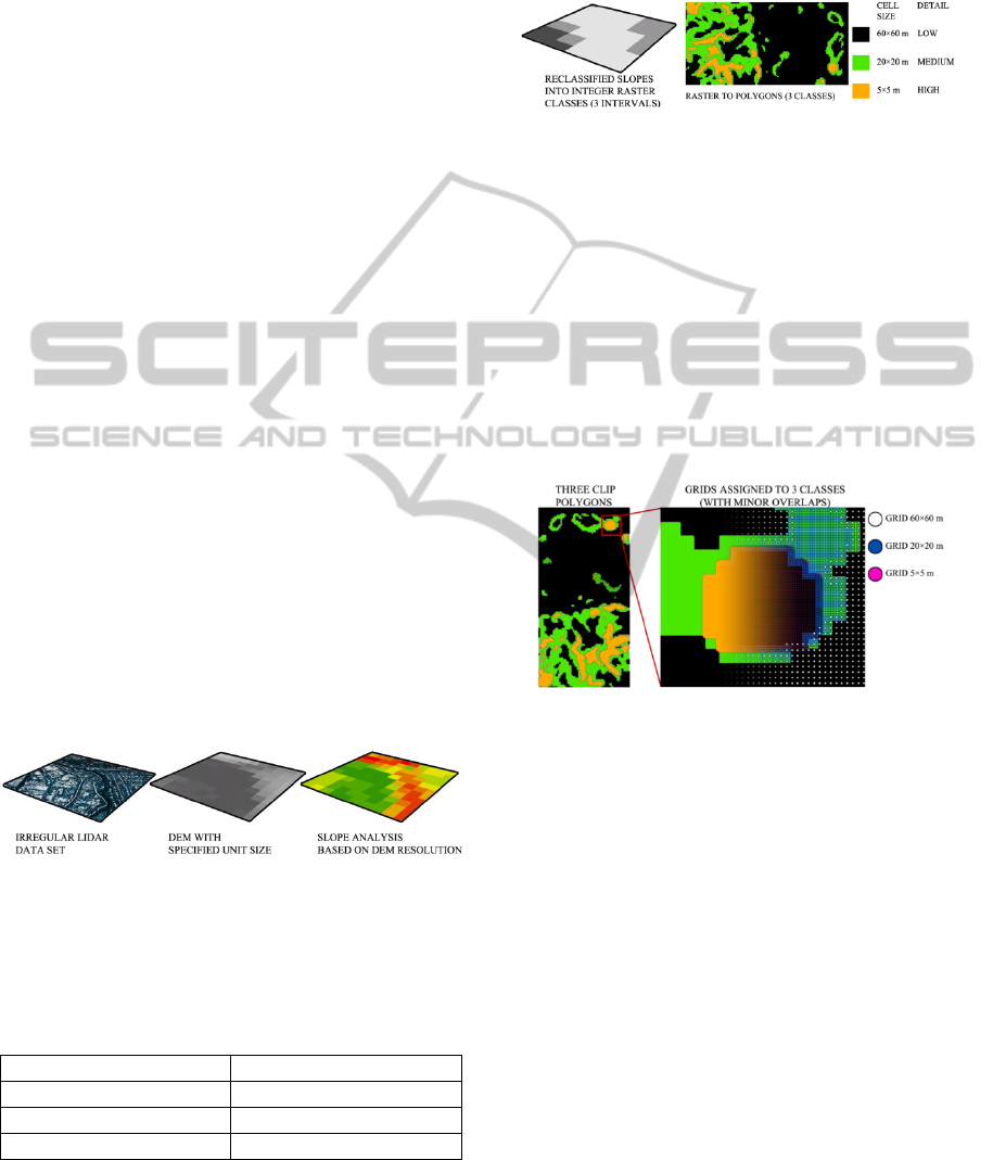
The main steps can be summarized as following.
Irregular LIDAR data set is converted to raster form
(DEM). This conversion is targeted to adequate cell
size and based on chosen method (e. g. most
frequent, mean,). Precision in the preservation of
real-measured values decreases but it is sufficient for
finding the outlines for all grids. In the next step the
slope analysis is performed. Quality of analysis is
based on the DEM cell size. Slope tool calculates the
maximum rate of change between each cell in the
raster and its eight neighbours.
These steps are shown magnified to recognize
cell size, on the Figure 7.
Figure 7: Slope analysis based on DEM.
To simplify the situation, ranges are aggregated into
3 groups (the same number of used grids). Flat,
semi-steep and steep regions (Table ).
Table 1: Aggregated ranges.
Slope class Gradient [%]
Flat region 0-20
Semi-steep region 21-35
Steep region >36
Decimal values of the raster are converted to
integers. This operation is prerequisite for raster to
polygon conversion. This conversion is made in high
precision to match individual outlines without blank
spaces. The process can be adjusted according to the
terrain type. Mainly by slope requirements, norms or
by DEM cell sizes (Figure 8).
Figure 8: Polygons used to clip interpolated grids.
Minor buffer can be also applied to each polygon
class to extend the boundary. This boundary will
provide an easier intersection of reconstructed
surfaces.
The final step in data preparation is to clip each
selected grid with associated polygon - 5×5 m grid
with orange coloured polygon, 20×20 m grid with
green polygon and 60×60 m with black polygon.
Some overlaps are apparent along the outlines of
each class. These overlaps will work like
intersection areas in the future research which will
utilize these data files for 3D scripting (Figure 9).
Figure 9: Assigned grids based on the slope analysis.
5 DISCUSSION
AND CONCLUSIONS
This section summarizes the results and outlines
possible ways forward in the future research.
5.1 Discussion
Authors performed a hybrid method of DTM
creation. This method is based on the classification
and segmentation of interpolated grids by chosen
method (IDW and Renka-Cline). This method
should lower hardware requirements by lowering the
resolution in certain areas and increasing the
resolution in high slope locations. Adaptive slope
adjustment of the interpolated grid resolution in
certain topographic locations can increase
reconstructed DTM dimensions significantly. This
SlopebasedGridCreationusingInterpolationofLIDARDataSets
231

study is based on the previous research where
authors explained parametric and procedural
visualisation which is built on the single grid with
constant resolution. Output from the previous
research with constant grid can be demonstrated by
following figure and will be very similar even in this
study but in much larger area (Figure 10).
Figure 10: Constant grid used in 3D visualisation in
previous research (Processed in 3D Studio Max).
The future work will be directed to area of 3D
scripting (Maxscript). Set of XYZ files - interpolated
grids will be processed in 3D environment (3D
Studio Max). Each of chosen grids will form
quadrilateral polygonal surface. By help of
parametric, procedural and set operations, the DTM
will be fitted by a set of models to form digitized
photo realistic 3D polygonal version of terrain
model. Real-world attributes (height, density,
coordinates and sizes) will be maintained along with
possibility to combine all features with analyses.
5.2 Conclusions
The main goal and partial steps are completed
successfully. Solution of these steps, however,
resulted in other issues which will be further
explained in following research. These issues are
mentioned in the discussion. Results can be used for
example for simplifying computational tasks related
to LIDAR car control by means of substitution of
point cloud by DTM which provides faster results.
ACKNOWLEDGEMENTS
This work was supported by the project No.
CZ.1.07/2.2.00/28.032 Innovation and support of
doctoral study program (INDOP), financed from EU
and Czech Republic funds.
REFERENCES
Axelsson, P., 2000. DEM generation from laser scanner
data using adaptive TIN models, International Archive
of Photogrammetry and Remote Sensing, 33 (B4),
110-117.
Belka, L., 2012. Airborne laser scanning and production of
the new elevation model in the Czech Republic,
Vojenský geografický obzor, 55 (1), 19-25.
Klimanek, M., 2006. Optimization of digital terrain model
for its application in forestry, Journal of Forest
Science, 52 (5), 233-241.
Li, J., Taylor, G., Kidner, D. and Ware, M., 2008.
Prediction and visualization of GPS multipath signals
in urban areas using LIDAR Digital Surface Models
and building footprints, International Journal of
Geographical Information Science, 22 (11-12), 1197-
1218.
Longley, P., A. et al., 2011. Geographic Information
Systems and Science, 3,539
Mandlburger, G., Hauer, C., Hofle, B., Habersack, H. and
Pfeifer, N., 2009. Optimization of LIDAR derived
terrain models for river flow modeling, Hydrology and
Earth System Sciences, 1453-1466.
Renka, R. J. and Cline, A. K., 1984. A triangle-based C
Interpolation Method. Journal of Mathematics, 14,
223-237.
ICSOFT2013-8thInternationalJointConferenceonSoftwareTechnologies
232
