GREEN-PSO: Conserving Function Evaluations

in Particle Swarm Optimization

Stephen M. Majercik

Department of Computer Science, Bowdoin College, Brunswick, Maine, U.S.A.

Keywords:

Particle Swarm Optimization, Swarm Intelligence.

Abstract:

In the Particle Swarm Optimization (PSO) algorithm, the expense of evaluating the objective function can

make it difﬁcult, or impossible, to use this approach effectively; reducing the number of necessary function

evaluations would make it possible to apply the PSO algorithm more widely. Many function approximation

techniques have been developed that address this issue, but an alternative to function approximation is func-

tion conservation. We describe GREEN-PSO (GR-PSO), an algorithm that, given a ﬁxed number of function

evaluations, conserves those function evaluations by probabilistically choosing a subset of particles smaller

than the entire swarm on each iteration and allowing only those particles to perform function evaluations. The

“surplus” of function evaluations thus created allows a greater number of particles and/or iterations. In spite of

the loss of information resulting from this more parsimonious use of function evaluations, GR-PSO performs

as well as, or better than, the standard PSO algorithm on a set of six benchmark functions, both in terms of the

rate of error reduction and the quality of the ﬁnal solution.

1 INTRODUCTION

Swarm intelligence is a natural phenomenon in which

complex behavior emerges from the collective activi-

ties of a large number of simple individuals who inter-

act with each other and their environment in very lim-

ited ways. A number of swarm based optimization

techniques have been developed, among them Parti-

cle Swarm Optimization (PSO). PSO, introduced by

Kennedy and Eberhart, is loosely based on the phe-

nomenon of birds ﬂocking (Kennedy and Eberhart,

1995). Virtual particles “ﬂy” through the solution

space in search of high quality solutions. The search

trajectory of a particle is inﬂuenced by both the best

solution it has found so far (personal best) and the best

solution that has been found so far in its neighbor-

hood; that solution will be a global best if the neigh-

borhood is the entire swarm (as in the original PSO

algorithm), or a local best if the neighborhood is a

strict subset of the swarm. The algorithm iteratively

updates the velocities and positions of the particles

guided by the personal bests and the neighborhood

bests, converging on a (hopefully) global optimum.

PSO is one of the most widely used swarm-based al-

gorithms and has been applied successful to many real

world problems (Poli et al., 2007). Many variants of

the PSO algorithm have been proposed (Sedighizadeh

and Masehian, 2009).

The trajectories of the particles in PSO depend crit-

ically on calculating the value of the objective func-

tion at every position each particle visits. In the stan-

dard PSO algorithm, every particle does a function

evaluation on every iteration in order to determine

the ﬁtness of the candidate solution at the particle’s

new position. A typical PSO algorithm uses at least

20-40 particles and thousands of iterations to ﬁnd

even a suboptimal (but acceptable) solution, and this

high number of function evaluations can be difﬁcult

to achieve in real world applications if the objective

function is expensive to compute, in terms of time

and/or money. For example, evaluating the effective-

ness of a complex control mechanism that a PSO al-

gorithm is trying to optimize might involve running a

simulation that takes several hours.

A common way of addressing this problem

is to use function approximation, which can take

many forms: response surface methods, radial ba-

sis functions, Kriging (DACE models), Gaussian pro-

cess regression, support vector machines, and neu-

ral networks (Landa-Becerra et al., 2008). An-

other approximation technique is ﬁtness inheritance,

in which the objective function value, or ﬁtness,

of an individual is approximated based on the ﬁt-

nesses of one or more other individuals designated as

160

M. Majercik S..

GREEN-PSO: Conserving Function Evaluations in Particle Swarm Optimization.

DOI: 10.5220/0004555501600167

In Proceedings of the 5th International Joint Conference on Computational Intelligence (ECTA-2013), pages 160-167

ISBN: 978-989-8565-77-8

 2013 SCITEPRESS (Science and Technology Publications, Lda.)

“parents”(Reyes-Sierra and Coello Coello, 2007).

Instead of using less expensive—but possibly less

effective—approximations of the function, an algo-

rithm could perform fewer exact evaluations of the

function, thereby conserving this resource. This is the

approach adopted by GREEN-PSO (GR-PSO), the algo-

rithm we present here. GR-PSO demonstrates that per-

formance comparable to or, in some cases, better than

that of the standard PSO algorithm can be achieved by

permitting only a subset of the particles in the swarm

to do function evaluations during each iteration, and

using the conserved function evaluations to increase

the number of particles in the swarm and/or the num-

ber of iterations that are possible, given a ﬁxed num-

ber of function evaluations.

In Section 2, we describe the basic PSO algorithm

and present the GR-PSO algorithm. We describe and

discuss the results of our experiments in Section 3.

We discuss related work in Section 4, and conclude

with some ideas for future work in Section 5.

2 PSO AND GR-PSO

2.1 Standard PSO

The standard PSO algorithm uses a swarm of particles

to iteratively search a d-dimensional solution space

for good solutions, guided by their own experience

and that of the swarm. The number of particles in the

swarm is ﬁxed and the position and velocity of each

particle i, ~x

and ~v

, respectively, are initialized ran-

domly. Particle i remembers the best solution it has

found so far, ~p

, and the best solution found so far

by the particles in particle i’s neighborhood, ~g

. (In

the original PSO algorithm, the neighborhood of ev-

ery particle is the entire swarm.) The velocity ~v

particle i is updated during each iteration such that

its motion is biased toward both ~p

and ~g

, and the

new velocity is used to update its position ~x

. There

are a number of basic PSO algorithms. For purposes

of comparison, we adopt the PSO algorithm with a

constriction coefﬁcient χ and velocity limits as de-

scribed in (Poli et al., 2007), which we reproduce here

with minor changes. The velocity and position update

equations are:

← χ(~v

U(0, φ

) ⊗(~p

−~x

) +

U(0, φ

) ⊗(~g

−~x

))

(1)

←~x

+~v

(2)

where:

• φ

and φ

, the acceleration coefﬁcients that scale

the attraction of particle i to ~p

and ~g

, respec-

tively, are equal,

•

U(0, φ

) is a vector of real random numbers uni-

formly distributed in [0, φ

], which is randomly

generated at each iteration for each particle, and

• ⊗ is component-wise multiplication.

The value of the constriction coefﬁcient χ is:

φ−2+

√

−4φ

where φ = φ

+ φ

= 4.1, giving χ a

value of approximately 0.7298. Finally, each compo-

nent ~v

is restricted to a range [V

min

max

], where V

min

and V

max

are the minimum and maximum values of

the search space and are identical for each dimension.

2.2 GR-PSO

The PSO algorithm is often motivated by referencing

the human decision-making process, in which an in-

dividual, confronted with a problem, makes a deci-

sion based partially on her own experience solving

that problem in the past and partially on the experi-

ence of others who have solved that problem before.

Extending that analogy, we suggest that, while trying

to improve the best solution she has found in the past,

she may suspend evaluation of her efforts for a period

of time, in order to conserve the resources that would

be required to evaluate the solution. A second goal

might be to prevent evaluating a new solution prema-

turely and possibly rejecting it before its value can be

accurately assessed.

GR-PSO models these goals in the following way.

GR-PSO operates like S-PSO, except that each parti-

cle, after calculating a new velocity and changing its

position according to that velocity, performs a func-

tion evaluation on its new position with some proba-

bility probFE, where 0.0 < probFE < 1.0. This means

that on every iteration, the expected number of par-

ticles doing a function evaluation is (n × probFE),

where n is the number of particles in the swarm, so

the expected number of iterations is (numFEs/(n ×

probFE)), where numFEs is the total number of func-

tion evaluations available. This allows the swarm to

use more particles for the same number of iterations,

or more iterations for the same number of particles.

See Figure 1 for pseudocode for GR-PSO.

3 EXPERIMENTAL RESULTS

We tested GR-PSO on six standard benchmark func-

tions: Sphere ( f

), Rosenbrock ( f

), Ackley ( f

Griewank ( f

), Rastrigin ( f

), and Penalized Function

P16 ( f

) ( f

identiﬁers used in Tables 1 and 2). See

(Bratton and Kennedy, 2007) for the function deﬁni-

tions. Sphere and Rosenbrock are uni-modal func-

tions, while Ackley, Griewank, Rastrigin, and Pe-

GREEN-PSO:ConservingFunctionEvaluationsinParticleSwarmOptimization

161

BEGIN

Initialize swarm

while (numFunctionEvaluations ≤ 10,000)

for each particle:

Calculate velocity and move

if (randomDouble < probFE)

Evaluate new position and update bests

end-if

end-for

end-while

END

Figure 1: Pseudocode for GR-PSO.

nalized Function P8 are multi-modal functions with

many local optima. The optimum (minimum) value

for all of these functions is 0.0. We randomly shifted

the location of the optima away from the center of

the search space in order to avoid the tendency of

PSO algorithms to converge to the center (Monson and

Seppi, 2005).

We tested each of these functions in 30 dimen-

sions. We used the gbest topology, in which the

neighborhood for each particle is the entire swarm,

for both GR-PSO and S-PSO. We ﬁxed the number of

function evaluations at 10,000 and tested over a range

of number of particles (10, 20, 50, 100, 200) and a

range of values for probFE (0.9, 0.8, . . . , 0.1). We

measured the mean and standard deviation of the best

(lowest) function value found and the median error

every 2,000 function evaluations (to avoid the effect

of outliers).

A note on our choice of topologies: It seems likely

that GR-PSO works, at least in part, because, by de-

laying the discovery of new global bests, it weakens

the tendency of the gbest topology to produce early

convergence on a local minimum. Topologies with

smaller neighborhoods, such as the ring topology (in

which the particles can be viewed as being arranged in

a ring, and the neighbors of each particle are just the

two particles on either side of it) also improve per-

formance by slowing the propagation of the global

best. And, in fact, it was the case that, using the

ring topology, GR-PSO did not provide the same per-

formance gains over S-PSO as it did with the gbest

topology. Thus, it would seem that a more appro-

priate comparison would be between GR-PSO using

the gbest topology and S-PSO using the ring topology.

The improved performance of the ring topology over

the gbest topology, however, is obtained only with a

sufﬁcient number of iterations and our limit of 10,000

function evaluations did not allow sufﬁcient iterations

for the ring topology’s beneﬁts to materialize. In fact,

while S-PSO with the ring topology outperformed S-

PSO with the gbest topology when 200,000 function

evaluations were allowed, S-PSO with the gbest topol-

ogy outperformed S-PSO with the ring topology when

only 10,000 function evaluations were allowed. For

this reason, we feel that the appropriate comparison

for GR-PSO with the gbest topology is still S-PSO with

the gbest topology, and we report those results.

Initial tests suggested that 10 particles are unable

to explore the space sufﬁciently, even given the addi-

tional iterations provided by a probFE of less than 1.0,

and that swarms of 100 or 200 particles reduce the

number of iterations (given the ﬁxed number of func-

tion evaluations) to unacceptable levels, in spite of the

additional iterations provided by a probFE of less than

1.0. Thus, we conﬁned further tests to 20-particle and

50-particle swarms. Initial tests of the S-PSO algo-

rithm over the same range of number of particles in-

dicated that 20-particle and 50-particle swarms were

best for that algorithm as well, for similar reasons.

Given a swarm with 20 or 50 particles, the im-

provement in performance was most pronounced at

or below a probFE of 0.5. The performance showed

a tendency to improve as probFE decreased, so we

tested two values below 0.1, i.e. 0.05 and 0.01. While

a probFE of 0.05 often produced results that were bet-

ter than those with a probFE of 0.1, a probFE of 0.01

was almost never better than a probFE of 0.05. In ad-

dition, since GR-PSO reduces the number of function

evaluations on each iteration by a factor of probFE,

the run time increases by a factor of 1/probFE, and the

additional run time with a probFE of 0.01 did not jus-

tify the occasional improvement in performance. The

best results for 20-particle and 50-particle swarms

were obtained with a probFE of 0.2, 0.1, or 0.05.

Thus, we show results for these six GR-PSO cases and

for S-PSO with 20 particles and 50 particles.

Results for the six versions of GR-PSO and the two

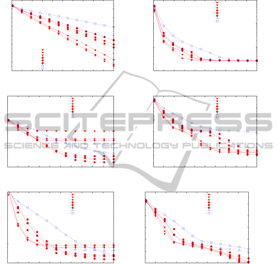
versions of S-PSO are presented in Table 1 and Fig-

ure 2. For each function, the results from the six GR-

PSO algorithms are followed by those from the two

S-PSO algorithms. The mean and standard deviation

of the lowest function value found are shown in Ta-

ble 1. To show the reduction in error during the run,

we report the median error at intervals of 2,000 func-

tion evaluations, also in Table 1. For each function, in

each column, the best result is in bold-face and is ital-

icized, and the two next best results are in bold-face.

In all cases, GR-PSO achieves the lowest av-

erage function value, and in all but three cases—

Rosenbrock ( f

), Ackley ( f

) and Rastrigin ( f

)—

the best three results are all achieved by GR-PSO.

With the exception of Ackley ( f

) and Rastrigin ( f

the algorithms with the best three average function

values also have the lowest standard deviations. In

three cases—Sphere ( f

), Griewank ( f

), and Penal-

IJCCI2013-InternationalJointConferenceonComputationalIntelligence

162

Table 1: Performance of GR-PSO and S-PSO over 121 runs.

Func- Mean Function Value Median Error (121 runs) for Num of Function Evaluations

tion Algorithm (Standard Deviation) 2,000 4,000 6,000 8,000 10,000

CPSO-20-0.2 5.44e-07 (2.36e-06) 1.47e+02 5.43e-01 1.88e-03 9.45e-06 3.09e-08

CPSO-20-0.1 4.91e-08 (2.11e-07) 8.61e+01 1.92e-01 4.66e-04 1.01e-06 2.83e-09

CPSO-20-0.05 1.31e-07 (1.22e-06) 5.66e+01 1.10e-01 2.48e-04 5.81e-07 1.24e-09

CPSO-50-0.2 1.77e-03 (2.40e-03) 8.61e+02 2.86e+01 8.01e-01 2.36e-02 8.25e-04

CPSO-50-0.1 1.65e-04 (2.04e-04) 5.76e+02 1.25e+01 2.49e-01 5.05e-03 8.85e-05

CPSO-50-0.05 3.70e-05 (4.74e-05) 4.41e+02 7.08e+00 8.35e-02 1.54e-03 1.95e-05

SPSO-20 5.42e-03 (1.28e-02) 6.70e+02 2.15e+01 9.19e-01 3.08e-02 9.94e-04

SPSO-50 1.14e+00 (1.47e+00) 2.93e+03 3.67e+02 4.73e+01 5.66e+00 6.93e-01

CPSO-20-0.2 3.77e+01 (2.42e+01) 8.88e+01 3.08e+01 2.75e+01 2.67e+01 2.62e+01

CPSO-20-0.1 3.45e+01 (2.47e+01) 7.15e+01 2.89e+01 2.72e+01 2.66e+01 2.61e+01

CPSO-20-0.05 3.57e+01 (2.56e+01) 7.66e+01 2.82e+01 2.70e+01 2.65e+01 2.61e+01

CPSO-50-0.2 3.11e+01 (1.57e+01) 1.35e+02 3.98e+01 2.84e+01 2.72e+01 2.67e+01

CPSO-50-0.1 3.52e+01 (2.10e+01) 1.29e+02 5.30e+01 2.85e+01 2.74e+01 2.68e+01

CPSO-50-0.05 3.06e+01 (1.67e+01) 1.12e+02 3.28e+01 2.79e+01 2.71e+01 2.65e+01

SPSO-20 3.24e+01 (1.80e+01) 1.28e+02 4.82e+01 2.89e+01 2.70e+01 2.60e+01

SPSO-50 4.04e+01 (2.44e+01) 2.86e+02 9.94e+01 4.36e+01 3.00e+01 2.80e+01

CPSO-20-0.2 9.93e+00 (8.00e+00) 7.85e+00 5.57e+00 5.53e+00 5.53e+00 5.53e+00

CPSO-20-0.1 9.92e+00 (7.50e+00) 7.78e+00 6.16e+00 6.13e+00 6.13e+00 6.13e+00

CPSO-20-0.05 1.17e+01 (7.36e+00) 1.21e+01 1.04e+01 1.02e+01 1.02e+01 1.02e+01

CPSO-50-0.2 6.04e+00 (8.72e+00) 8.60e+00 3.56e+00 1.76e+00 1.35e+00 1.34e+00

CPSO-50-0.1 7.48e+00 (9.23e+00) 8.91e+00 3.33e+00 1.94e+00 1.65e+00 1.65e+00

CPSO-50-0.05 8.54e+00 (9.18e+00) 8.41e+00 3.40e+00 2.25e+00 2.02e+00 2.01e+00

SPSO-20 9.39e+00 (8.15e+00) 9.36e+00 5.07e+00 4.59e+00 4.38e+00 4.38e+00

SPSO-50 8.35e+00 (9.08e+00) 1.30e+01 6.78e+00 4.08e+00 2.85e+00 2.35e+00

CPSO-20-0.2 3.78e-02 (6.66e-02) 2.01e+00 4.60e-01 2.65e-02 1.72e-02 1.72e-02

CPSO-20-0.1 8.09e-02 (2.95e-01) 1.59e+00 2.54e-01 3.55e-02 2.70e-02 2.70e-02

CPSO-20-0.05 6.67e-02 (1.63e-01) 1.69e+00 1.94e-01 2.56e-02 2.21e-02 2.21e-02

CPSO-50-0.2 1.72e-02 (1.97e-02) 9.26e+00 1.28e+00 8.24e-01 7.14e-02 1.23e-02

CPSO-50-0.1 1.74e-02 (2.54e-02) 7.39e+00 1.11e+00 4.50e-01 2.60e-02 1.08e-02

CPSO-50-0.05 1.85e-02 (2.17e-02) 4.81e+00 1.06e+00 1.92e-01 1.53e-02 9.93e-03

SPSO-20 9.02e-02 (1.67e-01) 6.65e+00 1.18e+00 5.17e-01 7.28e-02 3.99e-02

SPSO-50 6.93e-01 (2.32e-01) 3.16e+01 4.11e+00 1.38e+00 1.06e+00 7.09e-01

CPSO-20-0.2 1.02e+02 (4.88e+01) 1.07e+02 9.08e+01 9.05e+01 9.05e+01 9.05e+01

CPSO-20-0.1 1.18e+02 (7.05e+01) 1.17e+02 9.66e+01 9.65e+01 9.65e+01 9.65e+01

CPSO-20-0.05 1.25e+02 (8.01e+01) 1.07e+02 9.46e+01 9.45e+01 9.45e+01 9.45e+01

CPSO-50-0.2 7.53e+01 (3.35e+01) 1.83e+02 9.58e+01 7.42e+01 6.71e+01 6.57e+01

CPSO-50-0.1 8.16e+01 (3.44e+01) 1.65e+02 9.30e+01 7.82e+01 7.37e+01 7.36e+01

CPSO-50-0.05 8.49e+01 (4.69e+01) 1.40e+02 8.42e+01 7.33e+01 7.17e+01 7.16e+01

SPSO-20 8.80e+01 (3.17e+01) 1.70e+02 9.87e+01 8.59e+01 8.36e+01 8.36e+01

SPSO-50 7.65e+01 (2.57e+01) 2.61e+02 1.71e+02 1.16e+02 8.73e+01 7.35e+01

CPSO-20-0.2 4.71e-01 (1.01e+00) 5.70e+03 1.43e+01 3.04e+00 3.65e-01 1.16e-02

CPSO-20-0.1 4.61e-01 (9.55e-01) 1.38e+03 1.07e+01 2.14e+00 1.12e-01 1.11e-02

CPSO-20-0.05 4.76e-01 (9.58e-01) 3.39e+02 9.24e+00 1.71e+00 9.74e-02 1.10e-02

CPSO-50-0.2 2.59e-01 (6.13e-01) 1.99e+05 4.76e+01 7.96e+00 7.33e-01 5.43e-02

CPSO-50-0.1 2.53e-01 (7.12e-01) 1.04e+05 2.66e+01 3.27e+00 2.32e-01 1.57e-02

CPSO-50-0.05 1.12e-01 (4.18e-01) 5.95e+04 2.57e+01 3.17e+00 1.34e-01 1.15e-02

SPSO-20 2.24e+00 (3.41e+00) 5.95e+04 2.44e+01 6.83e+00 2.21e+00 5.92e-01

SPSO-50 4.38e+00 (5.76e+00) 8.52e+05 2.57e+03 3.32e+01 9.27e+00 2.33e+00

Key: CPSO-n-p = GR-PSO with n particles and probFE = p SPSO-n = S-PSO with n particles

GREEN-PSO:ConservingFunctionEvaluationsinParticleSwarmOptimization

163

1e-10

1e-08

1e-06

0.0001

0.01

100

10000

1e+06

0 1000 2000 3000 4000 5000 6000 7000 8000 9000 10000

Median Absolute Value Error

Number of Function Evaluations

SPHERE FUNCTION

CFE-PSO, 20, 0.20

CFE-PSO, 20, 0.10

CFE-PSO, 20, 0.05

CFE-PSO, 50, 0.20

CFE-PSO, 50, 0.10

CFE-PSO, 50, 0.05

S-PSO, 20

S-PSO, 50

(a) Sphere Function

100

1000

10000

0 1000 2000 3000 4000 5000 6000 7000 8000 9000 10000

Median Absolute Value Error

Number of Function Evaluations

ROSENBROCK FUNCTION

CFE-PSO, 20, 0.20

CFE-PSO, 20, 0.10

CFE-PSO, 20, 0.05

CFE-PSO, 50, 0.20

CFE-PSO, 50, 0.10

CFE-PSO, 50, 0.05

S-PSO, 20

S-PSO, 50

(b) Rosenbrock Function

100

0 1000 2000 3000 4000 5000 6000 7000 8000 9000 10000

Median Absolute Value Error

Number of Function Evaluations

ACKLEY FUNCTION

CFE-PSO, 20, 0.20

CFE-PSO, 20, 0.10

CFE-PSO, 20, 0.05

CFE-PSO, 50, 0.20

CFE-PSO, 50, 0.10

CFE-PSO, 50, 0.05

S-PSO, 20

S-PSO, 50

0.001

0.01

0.1

100

1000

0 1000 2000 3000 4000 5000 6000 7000 8000 9000 10000

Median Absolute Value Error

Number of Function Evaluations

GRIEWANK FUNCTION

CFE-PSO, 20, 0.20

CFE-PSO, 20, 0.10

CFE-PSO, 20, 0.05

CFE-PSO, 50, 0.20

CFE-PSO, 50, 0.10

CFE-PSO, 50, 0.05

S-PSO, 20

S-PSO, 50

(d) Griewank Function

100

0 1000 2000 3000 4000 5000 6000 7000 8000 9000 10000

Median Absolute Value Error

Number of Function Evaluations

RASTRIGIN FUNCTION

CFE-PSO, 20, 0.20

CFE-PSO, 20, 0.10

CFE-PSO, 20, 0.05

CFE-PSO, 50, 0.20

CFE-PSO, 50, 0.10

CFE-PSO, 50, 0.05

S-PSO, 20

S-PSO, 50

(e) Rastrigin Function

0.01

100

10000

1e+06

1e+08

1e+10

0 1000 2000 3000 4000 5000 6000 7000 8000 9000 10000

Median Absolute Value Error

Number of Function Evaluations

PENALIZED FUNCTION P16

CFE-PSO, 20, 0.20

CFE-PSO, 20, 0.10

CFE-PSO, 20, 0.05

CFE-PSO, 50, 0.20

CFE-PSO, 50, 0.10

CFE-PSO, 50, 0.05

S-PSO, 20

S-PSO, 50

(f) Penalized Function P16

Figure 2: Comparison of GR-PSO and S-PSO: median absolute value error (log scale) as a function of number of function

evaluations.

ized P16 ( f

)—the two S-PSO algorithms have the

worst average function values.

In the case of Sphere ( f

), the average function

value of the best GR-PSO algorithm (20 particles and

probFE of 0.1) was ﬁve orders of magnitude better

than that of the best S-PSO algorithm (20 particles).

And, in the case of Penalized P16 ( f

), the average

function value of the best GR-PSO algorithm (50 par-

ticles and probFE of 0.05) was an order of magnitude

better than that of the best S-PSO algorithm (20 parti-

cles). In the other four functions, the performance of

the best GR-PSO algorithm and the best S-PSO algo-

rithm had the same order of magnitude, but we feel

that the proper perspective here is not that the dif-

ference is small, but that, in spite of not performing

function evaluations at every opportunity, even to the

point where the expected number of particles doing a

function evaluation during an iteration was only one

particle (20 particles with a probFE of 0.05), the per-

formance of GR-PSO was no worse than S-PSO.

IJCCI2013-InternationalJointConferenceonComputationalIntelligence

164

Final median error showed similar results, with

GR-PSO showing the lowest median error in all

cases but Rosenbrock ( f

). In all but two cases—

Rosenbrock ( f

) and Rastrigin ( f

)—the algorithms

that achieved the three lowest ﬁnal median errors were

GR-PSO algorithms. And at every function evalua-

tion milestone, the algorithms with the three lowest

median error were all GR-PSO algorithms. More im-

portantly, the best GR-PSO algorithm reduced the me-

dian error more quickly in two cases—Sphere ( f

)

and Grieweank ( f

)—than the best S-PSO algorithm

(Figure2). In Sphere ( f

), this was true throughout the

run, and in Grieweank ( f

), this was true from approx-

imately function evaluation 3000 to function evalua-

tion 5500. (See Figure 2.)

None of the six GR-PSO algorithms tested was the

best in all cases, but the results indicate that, over the

range of values we tested, the number of particles is

a more signiﬁcant factor than the value of probFE;

for all the functions, changing the value of probFE

does not seem to make a signiﬁcant difference. With

the exception of Ackley ( f

), the 20-particle GR-PSO

has better performance than the 50-particle GR-PSO,

in terms of median error, until at least approximately

function evaluation 3,500. For the Sphere Function

( f

), that difference persists throughout the run, and

for Griewank ( f

) and the Penalized Function P8 ( f

that difference persists until approximately function

evaluation 7500 and function evaluation 5500, respec-

tively. Thus, these results suggest that while a mini-

mum number of particles is necessary to explore the

solution space (more than 10, given our initial explo-

rations described above), a smaller swarm can explore

the space sufﬁciently, and the increased number of it-

erations made possible by the smaller swarm, more

than compensates for the size of the swarm.

The ﬁnal errors for the 121 runs for the best

GR-PSO algorithm and the best S-PSO algorithm for

each function were rank ordered and a 2-tailed Mann-

Whitney U-test was used to compare the ranks. Since

the samples were large enough (> 20), the distribution

of the U statistic approximates a normal distribution,

so we report the Z-score, which is typically used in

such cases, as well as the U-score. The results indi-

cate a statistically signiﬁcant difference in the distri-

butions of the two groups at the 0.01 level—the error

of the GR-PSO tests being less than that of the S-PSO

tests—for four of the test functions: Sphere ( f

), Ack-

ley ( f

), Griewank ( f

), and Penal P16 ( f

). The re-

sults indicated that there was not a statistically signif-

icant difference for two of the functions: Rosenbrock

( f

) and Rastrigin ( f

). See Table 2.

GR-PSO can be viewed as an extreme form of ﬁt-

ness inheritance, so we also compared GR-PSO to a

Table 2: Mann-Whitney statistics for ﬁnal errors.

Mean Rank

Fnc GR-PSO S-PSO U Z p

60.5 181.0 1 -13.44 0.0

119.6 123.5 7084 -0.43 0.67

93.3 149.7 3913 -6.26 0.0

90.5 152.5 3570 -6.89 0.0

115.5 127.5 6592 -1.34 0.18

85.6 157.4 2977 -7.98 0.0

PSO algorithm that employs this approach. In ﬁt-

ness inheritance techniques, the value of the objective

function for a particle’s current position is approxi-

mated based on the objective function values of some

set of particles designated as its “parents,” thereby

avoiding function evaluations. In GR-PSO, a particle

that does not do a function evaluation is its own par-

ent, inheriting its own function evaluation directly.

Reyes-Sierra and Coello Coello incorporated ﬁt-

ness inheritance into a PSO algorithm (the only work

we are aware of that incorporates ﬁtness inheritance

into the PSO algorithm) and tested the effectiveness of

twelve ﬁtness inheritance techniques (and four ﬁtness

approximation techniques) in a multi-objective PSO

algorithm (Reyes-Sierra and Coello Coello, 2007).

MOPSO, the multi-objective PSO algorithm they test

these techniques on, is based on Pareto dominance

and, at any given point, there is a set of leaders, which

are the nondominated solutions. The scope from

which these leaders are drawn is the entire swarm, so

the topology of their algorithm is similar to the global

topology of GR-PSO.

These leaders, along with the standard personal

best of a particle and the previous position of a par-

ticle, form the set of possible parents when calculat-

ing the ﬁtness inherited by that particle. We com-

pared GR-PSO to the best three techniques (accord-

ing to their ranking of overall performance). To apply

these techniques in a single objective setting, we used

the global best for any situation in which a particle

from the set of leaders was called for.

The performance of all three of these approaches

was never better than the best GR-PSO population-

probability combinations, and, for all functions, the

majority of GR-PSO population-probability combina-

tions was better than all three of these techniques. We

note that the differences in performance were, in some

cases, quite small. We are not claiming that GR-PSO

is signiﬁcantly better than these three techniques, but

that these three techniques do not seem to be better

than GR-PSO.

It is interesting to note, that the probabilities they

tested were equivalent to GR-PSO probabilities in the

GREEN-PSO:ConservingFunctionEvaluationsinParticleSwarmOptimization

165

range of [0.6, 0.9], much higher than the function eval-

uation probabilities we found to be best, i.e. in the

range of [0.05, 0.2]. This supports the idea that in

a larger neighborhood, such as the gbest topology,

it may be better to do without any information for

longer periods of time than to use the currently avail-

able information, even to approximate objective func-

tion values.

4 ADDITIONAL RELATED

WORK

As noted in Section 1, there are a number of tech-

niques that seek to avoid expensive function evalu-

ations by approximating the value of the objective

function. These techniques are catalogued and de-

scribed in (Landa-Becerra et al., 2008) for multi-

objective evolutionary algorithms. Since these tech-

niques have been used primarily in evolutionary algo-

rithms and since the GR-PSO approach is much more

closely related to the approximation technique of ﬁt-

ness inheritance, we will not discuss them further.

The work of Reyes-Sierra and Coello Coello is the

only work we know of that incorporates ﬁtness inher-

itance into a PSO algorithm; that work has been dis-

cussed in the previous section.

Akat and Gazi describe a decentralized, asyn-

chronous approach that allows the PSO algorithm to

be implemented on multiple processors with very

weak requirements on communication between those

processors (Akat and Gazi, 2008a). Particles reside

on different machines. At each time step, each par-

ticle has access only to some subset of those ma-

chines/particles; thus, there may be signiﬁcant inter-

vals during which a particle p has received no infor-

mation from particle p

; it may even be the case that,

on a given iteration, a particle receives no informa-

tion from any other particles, in which case its posi-

tion and velocity remain the same. They report that

the performance of their approach was comparable to

standard PSO implementations.

In other work, Akat and Gazi compared three ap-

proaches to creating dynamic neighborhoods and sug-

gested that all three approaches were viable alterna-

tives to static neighborhoods (Akat and Gazi, 2008b).

More importantly, however, they considered the effect

of the information ﬂow topology on the performance

of the algorithm. In the general case, the parameter

determining neighborhood composition for each ap-

proach is different for each particle, resulting in non-

reciprocal neighborhoods, which can be represented

as directed graphs. If these digraphs are strongly con-

nected over time, i.e. if there is a ﬁxed interval such

that the union of the digraphs over every interval of

iterations of that length is strongly connected, then

information ﬂow in the swarm will be preserved and

every particle eventually has access to the information

gathered by every other particle.

This work suggests the possibility that GR-PSO

is creating temporary, smaller neighborhoods, the in-

habitants of which are constantly changing, but that

are connected over time. Perhaps the probability of

doing a function evaluation is regulating the connect-

edness of these shifting neighborhoods. An investiga-

tion into this possibility could shed light on the per-

formance of GR-PSO and the performance of PSO al-

gorithms that use dynamic neighborhoods, in general.

Finally, our results suggest an intriguing relation-

ship with work of Garc

ıa-Nieto and Alba. In (Garc

ıa-

Nieto and Alba, 2012), they tested a variant of the

S-PSO algorithm in which the neighborhood for each

particle on each iteration is constructed by choosing

k other particles, or “informants,” randomly. They

tested the algorithm over a range of values for k and

found evidence for a quasi-optimal neighborhood size

of approximately 6. In a sense, the expected num-

ber of particles doing function evaluations in GR-PSO

during an iteration can be viewed as the number of

informants for every particle in each iteration, since

it is these particles that could potentially provide new

information. If we rank the performance of the GR-

PSO algorithms, and count the number of times each

one appeared in the top ﬁve best-performing algo-

rithms for each test function, we ﬁnd that the best

three are 20 particles with probFE of 0.2, 50 parti-

cles with probFE of 0.1, and 50 particles with probFE

of 0.05, with an expected number of particles doing

function evaluations on each iteration of 4, 5, and 2.5,

respectively. This suggests that there might be an op-

timal range for the expected number of particles do-

ing function evaluations during an iteration, and that

this range may be similar to the optimal range for the

number of informants in the work of Garc

ıa-Nieto and

Alba.

5 CONCLUSIONS AND FURTHER

WORK

We have presented GR-PSO, a PSO algorithm that

conserves function evaluations by probabilistically

choosing a subset of particles smaller than the entire

swarm on each iteration and allowing only those par-

ticles to perform function evaluations. The function

evaluations conserved in this fashion are used to in-

crease the number of particles in the swarm and/or the

number of iterations. In spite of the potential loss of

IJCCI2013-InternationalJointConferenceonComputationalIntelligence

166

information resulting from this restriction on the use

of function evaluations, GR-PSO performs as well as,

or better than, the standard PSO algorithm on a set of

standard benchmark functions.

GR-PSO also provides a novel way to control ex-

ploration and exploitation. Given a lower probability

of doing function evaluations, information about new

global and personal bests is delayed and the balance

is tipped away from exploitation toward exploration.

This opens up the possibility of using probFE as a

mechanism to dynamically adjust the relative levels

of exploration and exploitation in response to the be-

havior of the swarm.

The conservation technique we tested is very sim-

ple; there are many possibilities for more sophisti-

cated conservation mechanisms. It is possible that

adaptive approaches that take into account various

factors, such as the recent history of the particle and

the status of other particles in the particle’s neighbor-

hood, could improve performance. For example, per-

haps a particle should decide whether to skip a func-

tion evaluation based on the distance it has moved

and/or the change in its function value in the last k

moves. Another possibility that would still conserve

function evaluations, but allow particles to possibly

recover missed personal bests, would be for each par-

ticle to save the k most recent positions for which

it did not do a function evaluation, then pick one of

those randomly and evaluate it, adopting it as its per-

sonal best if it is better than its current personal best.

Perhaps more importantly, however, the idea of

conserving function evaluations suggests that it would

be fruitful to think of function evaluations as a

scarce resource that needs to be allocated over time.

This opens up the possibility of incorporating game-

theoretic mechanisms for resource allocation into the

PSO framework. For example, an auction mechanism

could be used to allocate function evaluations either to

individuals, or to neighborhoods that would, in turn,

allocate them to the individuals in those neighbor-

hoods. The amount of “money” that a particle has for

bidding purposes could depend on many things: for

example, how good its current solution is, the trend

of its personal best values, and the number of new

neighborhood bests it has been responsible for over

some period of time. A neighborhood could acquire

resources for bidding that depend on similar factors,

as well as how good its best is compared to the bests

of other neighborhoods.

REFERENCES

Akat, S. and Gazi, V. (2008a). Decentralized asynchronous

particle swarm optimization. In Swarm Intelligence

Symposium, 2008. SIS 2008. IEEE, pages 1 –8.

Akat, S. and Gazi, V. (2008b). Particle swarm optimization

with dynamic neighborhood topology: Three neigh-

borhood strategies and preliminary results. In Swarm

Intelligence Symposium, 2008. SIS 2008. IEEE, pages

1 –8.

Bratton, D. and Kennedy, J. (2007). Deﬁning a standard for

particle swarm optimization. In Swarm Intelligence

Symposium, 2007. SIS 2007. IEEE, pages 120–127.

Garc

ıa-Nieto, J. and Alba, E. (2012). Why six informants

is optimal in PSO. In Proceedings of the fourteenth

international conference on Genetic and evolutionary

computation conference, GECCO ’12, pages 25–32.

Kennedy, J. and Eberhart, R. (1995). Particle swarm opti-

mization. Proceedings of IEEE, pages 1942–1948.

Landa-Becerra, R., Santana-Quintero, L. V., and Coello

Coello, C. A. (2008). Knowledge incorporation in

multi-objective evolutionary algorithms. In Multi-

Objective Evolutionary Algorithms for Knowledge

Discovery from Databases, pages 23–46.

Monson, C. K. and Seppi, K. D. (2005). Exposing origin-

seeking bias in PSO. In GECCO, pages 241–248.

Poli, R., Kennedy, J., and Blackwell, T. (2007). Particle

swarm optimization: An overview. Swarm Intelli-

gence, 1:33–57.

Reyes-Sierra, M. and Coello Coello, C. A. (2007). A study

of techniques to improve the efﬁciency of a multi-

objective particle swarm optimizer. In Studies in Com-

putational Intelligence (51), Evolutionary Computa-

tion in Dynamic and Uncertain Environments, pages

269–296.

Sedighizadeh, D. and Masehian, E. (2009). Particle swarm

optimization methods, taxonomy and applications. In-

ternational Journal of Computer Theory and Engi-

neering, 1(5):486–502.

GREEN-PSO:ConservingFunctionEvaluationsinParticleSwarmOptimization

167