
Gait Optimization of a Rolling Knee Biped at Low Walking Speeds
Mathieu Hobon
1
, Nafissa Lakbakbi Elyaaqoubi
2
and Gabriel Abba
2
1
Design Manufacturing and Control Laboratory (LCFC), Arts et Mtiers ParisTech CER Metz,
4 rue Augustin Fresnel, 57078 Metz, France
2
Design Manufacturing and Control Laboratory (LCFC), National Engineering College of Metz,
1 route d’Ars Laquenexy, 57035 Metz Cedex, France
Keywords:
Walking Robot, Optimization Gait, Parametric Trajectory, Knee Kinematic.
Abstract:
This paper addresses an optimization problem of trajectories for a biped robot with a new modelled structure of
knees which is called rolling knee (RK). The first part of article is to present the new kinematic knee on a biped
robot and the different models used to know the dynamic of the robot during a walking step. The gait is cyclic
and simplified by a Single Support Phase (SSP) followed by an impact. The second part is a comparison of
the influence of the gait trajectory on the control, using cubic spline functions as well as the B´ezier functions.
The energetic criterion is minimized through optimization while using the simplex algorithm and the Lagrange
penalty functions to meet the constraints of stability and deflection of mobile foot. The main result is the using
of B´ezier functions permit to improve the energy gain in slow walking speeds. These trajectories permit to the
biped robot to walk progressively without energy disturbance unlike those with cubic spline functions.
1 INTRODUCTION
On a biped robot, the knee joints are classically re-
alized by revolute joints. Biomechanical studies talk
about the human knees that relate the movement of
this articulation which is a combination of a rota-
tion and a translation. (Hamon and Aoustin, 2010)
propose knee structures combining these movements
with a cross four-bar linkage. The simulations show
less energy usage through this solution comparing to
classical revolute joint knees. Another knee mecha-
nisms designed by (Van Oort et al., 2011) uses a sin-
gularity of the mechanism to save the energy. When
the mobile leg is stretched at the end of the step, the
knee is locked by the singularity and does not con-
sume energy during the next stance phase. The en-
ergy consumption also decreases during the gait. The
design of the knee mechanism in the LARP project in
(Gini et al., 2007) coming from studies on prosthetic
knees and consist of a structure with two cylinder sur-
faces in contact.
The walk is described by a succession of con-
tacts between feet and the ground. The important
issue is to keep the equilibrium of the biped during
this progression. Some control strategies need stable
reference trajectories to ensure the gait of the robot.
(Chevallereau et al., 2009), (Grizzle et al., 2001),
(Westervelt et al., 2001) introduce the stability of the
gait by studying the zero dynamics. The biped uses
reference trajectories to stabilize the zero dynamics.
The proposed method replaces the time variable by
a monotonic non-actuated variable depending on the
state X
e
of the robot. This variable is used to replace
time parametrizing the periodic motion of the biped.
Now, the problemis a constrained nonlinear optimiza-
tion problem where, the parameters of the desired tra-
jectories are found in order to minimize a criterion
defined by the integral-squared torque per step length.
Another method proposed by (Kajita et al., 2003) uses
reference trajectories of zero moment point (ZMP) to
control the stability of the biped during the walk. The
method defines a predictive control of the center of
mass and of the desired ZMP trajectories.
For a given kinematic structure of robot, the previ-
ous control laws have proven their viability when the
robot performsthe walking gaits at speeds of the order
of 0.5 to 1 m/s. Furthermore the robot is also used in
very different operating conditions and not only with
a constant gait speed. It is indeed necessary:
• To control the acceleration or deceleration phases
(see (Sabourin and Bruneau, 2005)).
• To planning feet trajectories, at slow walking
speeds, in an environment with moving obstacles
(Chestnutt et al., 2005).
• To generate the walking gaits at very low speed
207
Hobon M., Lakbakbi Elyaaqoubi N. and Abba G..
Gait Optimization of a Rolling Knee Biped at Low Walking Speeds.
DOI: 10.5220/0004457402070214
In Proceedings of the 10th International Conference on Informatics in Control, Automation and Robotics (ICINCO-2013), pages 207-214
ISBN: 978-989-8565-71-6
Copyright
c
2013 SCITEPRESS (Science and Technology Publications, Lda.)

for collaborative tasks like in (Evrard et al., 2009).
• To slow down speed when the robot starts chang-
ing direction like in (Wang et al., 2012).
The objective of our work is also to propose gait
support trajectories at low speeds. These trajectories
are based on a mathematical parametrized function.
We used B
´
ezier functions and cubic spline functions.
The optimization process of sthenic criterion provides
the vector of parameters for each function. The results
clearly show the advantages of B
´
ezier functions to ex-
press support trajectories at low speed. These results
are better than those proposed with spline functions in
(Hamon and Aoustin, 2010) and (Hobon et al., 2011)
for higher speed range.
In this paper, the simplex algorithm will be used
to demonstrate the advantage to utilize a rolling knee
structure in the design of biped robot.
The outline of the paper is following. In section 2,
the biped with the rolling knee structure is discussed.
The parametric gait is formulated in the section 3. The
section 4 introduces the optimization problem. Simu-
lations and results are presented in section 5. Finally,
section 6 presents the conclusion and perspectives.
2 MODEL
2.1 Biped Model
This study is focused on the cyclic walk of the biped
in the sagittal plane. The considered robot biped is
composed of seven rigid bodies with two feet, two
shins, two thighs and one trunk. The biped is all actu-
ated by six actuators. The objective is to compare the
performance of this robot using two trajectory func-
tions. The robot has revolute joints placed on hips
and ankles but the knee joints is composed of a struc-
ture called rolling knees and present in (Hobon et al.,
2011). Fig. 1 shows the robot studied with this con-
figuration. The rolling knee consists of a movement
of two cylindrical surfaces rolling without sliding, the
two surfaces are the terminal surface of the femur and
the tibia. The reference frame is ℜ
0
= (O
0
,~x
0
,~y
0
,~z
0
).
O
0
is defined by the projection of the point A
1
on the
ground. The direction of the walk is according to ~x
0
and ~z
0
the unit vector perpendicular to the ground.
The orientation of the links are defined by the ab-
solute angles q
i
,{i = 0... 6} referenced by the ver-
tical, the speed vector ˙q
i
,{i = 0.. .6} and the vector
Γ = [Γ
1
.. . Γ
6
]
T
which represents the torques placed
on the hips, the knees and the ankles (see Fig. 1). Fig.
2 shows the details of the knee configuration. The
contact between the femur and the tibia is maintained
with a bar on C
1
and C
2
of length r
1
+ r
2
with r
1
and
q
3
Cg
2
q
2
q
6
Cg
6
H
Cg
3
K
2
N
O
0
Cg
1
q
1
T
1
H
1
x
0
z
0
y
0
K
1
A
1
G
1
G
2
G
3
G
4
G
5
T
2
Cg
4
q
4
H
2
A
2
z
5
x
5
q
5
G
6
Figure 1: Biped robot with rolling joint knees.
r
2
are respectively the distance B
1
C
1
and B
2
C
2
. With
the rotation without sliding, we can write (1) and find
the relation of the angle γ
1
which shows the coupling
between the angles q
1
and q
2
for the leg support in
(2). Similarly for the mobile leg, γ
2
is the coupling
angle between q
3
and q
4
in 3.
B
1
K
1
= B
2
K
1
(1)
γ
1
=
r
1
q
1
+ r
2
q
2
r
1
+ r
2
(2)
γ
2
=
r
1
q
4
+ r
2
q
3
r
1
+ r
2
(3)
The dynamic model’s parameters are the length l
i
of the links for the robot, i = {0.. .6} and we have
an assumption gives us l
′
1
= A
1
C
1
= l
1
− r
1
and l
′
2
=
HC
2
= l
2
− r
2
, the position of the center of mass C
gi
,
the masses m
i
, the moments of inertia I
i
of each bodies
C
i
around the ~y
0
axis at C
gi
.
The coordinates of the hip, the heel and the toes
for the rolling knee configuration are:
x
H
= −l
′
2
sinq
2
− (r
1
+ r
2
)sinγ
1
− l
′
1
sinq
1
(4)
z
H
= l
′
2
cosq
2
+ (r
1
+ r
2
)cosγ
1
+ l
′
1
cosq
1
+ h
p
(5)
x
H
2
= x
H
+ l
′
2
sinq
3
+ lsinγ
2
+ l
′
1
sinq
4
−l
p
cos(q
5
) + h
p
sin(q
5
) (6)
z
H
2
= z
H
− l
′
2
cosq
3
− lcosγ
2
− l
′
1
cosq
4
−l
p
sin(q
5
) − h
p
cos(q
5
) (7)
x
T
2
= x
H
+ l
′
2
sinq
3
+ lsinγ
2
+ l
′
1
sinq
4
−(l
p
− L
p
)cos(q
5
) + h
p
sin(q
5
) (8)
ICINCO2013-10thInternationalConferenceonInformaticsinControl,AutomationandRobotics
208

g
1
q
1
q
2
C
2
z
2
x
1
z
1
r
2
C
1
r
1
B
2
B
1
K
1
x
2
Figure 2: Rolling knee of one leg.
z
T
2
= z
H
− l
′
2
cosq
3
− lcosγ
2
− l
′
1
cosq
4
−(l
p
− L
p
)sin(q
5
) − h
p
cos(q
5
) (9)
2.2 Dynamic Model
In this work, we consider only the walking gait de-
fined with Simple Support Phases (SSP) followed by
an impact between the mobile foot and the ground.
The impact produces the instantaneous exchange of
supporting leg during the gait. The dynamic model
for the SSP is assumed with the left leg on support.
Considering the gait like periodic with a permutation
of the legs at the impact, the study focuses on one step
beginning with the impact. The dynamic and impact
models are described as follow:
2.2.1 Dynamic Model During the SSP
The Lagrange equations are used to determine the
inverse dynamic model. Details are mentioned in
(Spong and Vidyasagar, 1991) and (Khalil and Dom-
bre, 2002). Posing q = [q
i
],i ∈ [0. ..6] and X
e
=
[q,x
H
,z
H
]
T
the state vector of dimension 9 × 1. The
inverse dynamic equation can be written as:
B A
c
L
(X
e
)
T
[Γ F
L
]
T
= D(X
e
)
¨
X
e
+H(
˙
X
e
,X
e
)+Q(X
e
)
(10)
with D(X
e
) represents the inertia matrix 9 × 9,
H(
˙
X
e
,X
e
) is the vector of Coriolis and centrifugal ef-
fects 9 × 1, Q(X
e
) is the vector of torques and forces
due to the gravity 9× 1 , B is the control matrix 9× 6
and A
c
L
(X
e
) is the Jacobian matrix 3× 9 of the foot
on support. The acceleration of ¨x
H
and ¨z
H
are cal-
culated with the hypotheses that the support foot re-
mains in contact during the SSP, x
A
1
= 0, z
A
1
−h
p
= 0
and q
0
= 0. By twice derivation to the state vector, we
obtain the constraint dynamic equations:
A
cL
(X
e
)
T
¨
X
e
+ H
cL
(X
e
) = 0 (11)
With the evolution of X
e
satisfying (11), the
torques Γ and external forces F
L
= [F
x
F
z
C
y
]
T
on the
stance ankle are calculated with (10) in any instant of
the gait.
2.2.2 Impact Model
During the gait, the left foot and then the right foot
alternatively touch the ground with a non zero speed.
This is the impact phase. The impact phase separates
two SSP. The contact phase between two rigid bod-
ies, the foot and the ground, produces a mechanical
energy dissipation phenomena (Pfeiffer and Glocker,
1996). We suppose that the restitution coefficient is
equal to zero. This assumption ensures that we have
no rebounds of the foot after the impact. The pro-
posed model is:
D(X
e
)
˙
X
e
+
−
˙
X
e
−
= A
T
c
L
I
R
(12)
A
c
L
(X
e
)
˙
X
e
+
= 0 (13)
∆
T
= D
−1
A
T
c
L
I
R
(14)
This model is used to find the speed vector af-
ter the impact
˙
X
e
+
from the configuration X
e
and the
speed vector before impact
˙
X
e
−
. ∆
i
is a vector (9× 1)
and is the difference between the speed after and be-
fore the impact for each axis i, i ∈ [0···6]. It will be
used to define the conditions of the trajectories in the
following section. This model also gives the impact
forces on the foot I
R
= [I
Fx
I
Fz
C
y
]
T
and the torque
applied on the ankle.
3 GAIT REFERENCE
PARAMETRIC TRAJECTORIES
Now, the gait is defined by the evolution of angular
coordinates of the bodies with respect to the time. The
goal is to find the best parametric trajectories to im-
prove the fluidity of the movement and to reduce the
energy consumption. The angular coordinates q
i
with
i = {0...6} can be parametrized by a cubic spline
function also, used in (Hamon and Aoustin, 2010),
(Banno et al., 2009) or order 3 B
´
ezier function of
(Westervelt et al., 2001), (Scheint et al., 2008). To
simplify the definition of the trajectories, the time
t is normalized to the dimensionless time variable
t
n
= t/T with T the step period. The gait can be
described by: at t
n
= 0, the left foot is fixed on the
GaitOptimizationofaRollingKneeBipedatLowWalkingSpeeds
209

ground and the right foot is behind the trunk. At
t
n
= 1, the right foot has an advance of a distance d
and it is in front of the trunk.
3.1 Cubic Spline Function
In this case, the trajectories are defined by two cubic
spline functions. Each function is parametrized for a
half-period. The knot vector has three knots so we
define t
k
= [0, 0.5, 1]. In neighbourhood of t
i
∈ t
k
,i =
[0,2], the spline function has the smoothness C
1
. We
suppose that at the timet
1
= 0.5, the second derivative
is continuous. Also, for t
0
= 0 and t
2
= 1, the impact
imposes a discontinuity on the velocities.
The expression of the cubic spline function is:
0 ≤ t
n
≤
1
2
→
f
q
i
(t
n
) =
3
j=0
a
i
j
t
j
n
(15)
1
2
≤ t
n
≤ 1
→
f
′
q
i
(t
n
) =
3
j=0
b
i
j
(1−t
n
)
j
(16)
where a
j
and b
j
are the eight parameters expressed
for each angle. Supposing k =
1
T
, the velocities and
accelerations are obtained by derivation:
˙q
i
(t) = k
d f
q
i
dt
n
(17)
¨q
i
(t) = k
2
d
2
f
q
i
dt
2
n
(18)
3.2 B
´
ezier Function
The trajectories now are defined by B
´
ezier function
and parametrized for one period from t
n
= 0 to t
n
= 1.
The function is C
2
on the interval ]0,1[. The parame-
ters c
i
j
are homogeneous to angular coordinates:
B
q
i
(t
n
) =
3
j=0
3!
j!(3− j)!
c
i
j
t
j
n
(1−t
n
)
(3− j)
(19)
where c
j
are the four parameters to describe each an-
gle q
i
(t) = B
q
i
(kt). The speeds and accelerations are
found by derivation.
3.3 Smoothness, Cyclicity and Vector of
Parameters
The study is focused on a cyclical gait defined by an
impact and SSP. We assume that the left foot is on
support during the SSP, also q
0
= 0. The unknown
vector q
i
is now for i = {1... 6}. Following hypothe-
ses are posed for the gait :
• The mobile foot is flat on the ground at the begin-
ning and at the end of the step
• The angles of the trunk and the mobile foot are
T-periodic
• The angles of the tibias and the thighs are 2T-
periodic
For the spline function, we consider the continuity
and the smoothness of the function at the half-period.
These conditions for the mobile foot, the trunk, the
tibias and the thighs lead to :
a
5
0
= b
5
0
= 0,a
5
2
= b
5
2
,a
5
3
= b
5
3
= −
4
3
a
5
2
(20)
a
6
0
= b
6
0
,a
6
2
= b
6
2
,a
6
3
= b
6
3
= −
4
3
a
6
2
(21)
a
1
0
= b
4
0
,a
1
2
= b
4
2
= a
4
2
+ 6(a
4
0
− a
1
0
),
b
1
3
= −6((a
1
0
− a
4
0
) +
4
3
(a
1
1
− a
1
2
)) (22)
a
4
0
= b
1
0
,a
4
2
= b
1
2
= a
1
2
+ 6(a
1
0
− a
4
0
),
b
4
3
= −6((a
4
0
− a
1
0
) +
4
3
(a
4
1
− a
4
2
)) (23)
a
2
0
= b
3
0
,a
2
2
= b
3
2
= a
3
2
+ 6(a
3
0
− a
2
0
),
b
2
3
= −6((a
2
0
− a
3
0
) +
4
3
(a
2
1
− a
2
2
)) (24)
a
3
0
= b
2
0
,a
3
2
= b
2
2
= a
2
2
+ 6(a
2
0
− a
3
0
),
b
3
3
= −6((a
3
0
− a
2
0
) +
4
3
(a
3
1
− a
3
2
)) (25)
The impact model imposes a relation between the
speed before and after the impact time for all mobile
bodies. For example, the speed of the right thigh after
the impact depend on (14) and on the speed of the left
thigh just before the impact. Theses conditions are
expressed as:
a
5
1
= b
5
1
+ ∆
5
(26)
a
6
1
= b
6
1
+ ∆
6
(27)
a
2
1
= b
3
1
+ ∆
2
(28)
a
3
1
= b
2
1
+ ∆
3
(29)
a
1
1
= b
4
1
+ ∆
1
(30)
a
4
1
= b
1
1
+ ∆
4
(31)
For the B
´
ezier function, the same conditions can
be expressed and we obtain:
c
i
0
= c
i
3
, i = [5,6] (32)
c
i
j
= c
i
(
3− j)
, i = [1, 4], j = [0,3] (33)
c
i
j
= c
i
(
3− j)
, i = [2, 3], j = [0,3] (34)
ICINCO2013-10thInternationalConferenceonInformaticsinControl,AutomationandRobotics
210

The impact model imposes for the B
´
ezier func-
tions :
c
5
1
= −3c
5
2
+ ∆
5
(35)
c
6
1
= 3(c
6
0
− c
6
2
) + ∆
6
(36)
c
2
1
= 3(c
2
0
− c
3
2
) + ∆
2
(37)
c
3
1
= 3(c
3
0
− c
2
2
) + ∆
3
(38)
c
1
1
= 3(c
1
0
− c
4
2
) + ∆
1
(39)
c
4
1
= 3(c
4
0
− c
1
2
) + ∆
4
(40)
The remaining parameters of the simplification are
equal to 17 for the cubic spline function. For those de-
fined in the B
´
ezier function, we identify 11 parameters
which are summarized in the table 1.
Table 1: Resume of vector of parameters.
Parametric function parameters
Cubic spline a
i
0
for i = {1,2,3,4,6},
function b
j
1
and a
j
2
for j = {1...6}
B
´
ezier articular c
i
0
for i = {1,2,3,4,6},
function c
j
2
for j = {1...6}
Finally, the parameters a
i
0
and c
i
0
which give
the initial angular position can be found with the
inverse geometric model of the Cartesian position
of the hip (x
H
(0),z
H
(0)). The period T is added
as parameter for the gait determination. The pa-
rameters vectors p
s
=[x
H
(0),z
H
(0),a
6
0
,b
j
1
,a
j
2
,T] and
p
b
=[x
H
(0),z
H
(0),c
6
0
,c
j
2
,T] are used in the following
optimization process.
In this section, we introduce two types of trajec-
tory functions to describe the gait. The cubic spline
function are parametrized by absolute angles, abso-
lute velocities and accelerations. The choice of pa-
rameters is sensitive to the walking speed and the ac-
celeration parameters introduces some convergence
problems. This motivates us to choose B
´
ezier func-
tions that are more homogeneous parameters corre-
sponding to absolute angles. Thus the smoothness
of the generated trajectories advantages the criterion
convergence.
4 OPTIMIZATION PROBLEM
The research of optimal parameters to produce the
best gait trajectories is challenging. The goal is to
search trajectories minimizing a criterion represent-
ing the energetic consumption of the robots while re-
specting the constraints due to the biped environment.
A gait is considered optimal if the gait is physically
feasible and with the minimal of power supply.
We have also to solve a nonlinear minimization
problem under constraints that can be expressed:
min
p
C
Γ
(p)
under Ψ(p) ≥ 0 with p = p
s
or p = p
b
(41)
with Ψ = [Ψ
1
Ψ
2
Ψ
3
Ψ
4
Ψ
5
Ψ
6
Ψ
7
]
T
are the constraints
imposed by the initial configuration of the robot and
the physical constraints considered before. The con-
straints are:
• Ψ
1
= F
z
define the vector of the force along the
z-axis and must be positive,
• Ψ
2
= x
ZMP
+ l
p
and Ψ
3
= −x
ZMP
+ (L
p
− l
p
) rep-
resent the limit position of the ZMP on x-axis
(ZMP must stay in the foot support) to guaranty
the stability of the robot,
• Ψ
4
= q
2
− q
1
and Ψ
5
= q
3
− q
4
are the choice
made to keep a gait human-like with no bend
backward of knees,
• Ψ
6
= z
H2
and Ψ
7
= z
T2
are used to have the z-
coordinates of heel and toes of the mobile foot
above the ground during the SSP.
The x-coordinates of ZMP is calculated by:
x
ZMP
=
Γ
1
− h
p
F
x
− m
p
s
x
g
F
z
(42)
The criterion used is the estimation of Joules
losses. It also named sthenic criterion (Tlalolini et al.,
2011) and defined by (43).
C
Γ
(p) =
2
d
T
0
Γ
T
Γ dt (43)
We propose to solve this problem by using the
Nelder-Mead simplex algorithm see (Lagarias et al.,
1998). This algorithm solves nonlinear problem with-
out constraints. The constraints are also added in the
criterion (43) as Lagrange multiplier. One of advan-
tages to use the simplex algorithm is the possibility
to explore the space around the initial vector. The
reloading of the obtained solution allows to avoid lo-
cal minima and also to converge to the optimal solu-
tion. The equation becomes:
C
Γ
(p) =
2
d
T
0
Γ
T
Γ+K
7
i=1
(e
(|Ψ
i
|−Ψ
i
)
−1) dt+Err
(44)
with Γ calculated from (10), Ψ
i
represents the con-
straints already defined, K is the multiplier of La-
grange equal to 10
6
in our calculation and Err can
handle the errors due to the inverse geometric model.
At the end of the optimization, we verify that the con-
straints are positive and Err are equal to zero in all
cases.
GaitOptimizationofaRollingKneeBipedatLowWalkingSpeeds
211
5 SIMULATIONS AND RESULTS
The simulations were done with the geometrical and
dynamic parameters of HYDROID Robot. The height
of this biped robot is 1.39m with a total mass of 45.36
kg. The table 2 in appendix gives the physical pa-
rameters of each body part of this robot. For these
simulations, the radii r
1
and r
2
are chosen equal to
5 cm. The objective of the simulation is to acquire
the best trajectory function for the configuration de-
fined in 2 and to find the best solution. Two series of
optimization were done following the mathematical
expressions defined in 3. We will observe the evolu-
tion of criteria and compare the angles, the velocities
and joint torques. We will examine the evolution of
the convergence criterion during optimization phases
using the cubic spline functions and the B
´
ezier func-
tions.
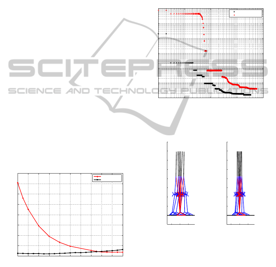
In Fig. 3, the evolution of optimal criteria versus
the walking speed is presented between 0.1 m/s to 0.3
m/s. The criteria with the B
´
ezier functions are lower
than the one with the cubic spline functions and the
criterion gain is about 96% for the walking speed at
0.1 m/s, it is about 68% at 0.2 m/s. The progression
of the criterion using the B
´
ezier functions increases
slightly. It is an advantage to starting up of the walk of
a biped robot compared to the use of the cubic spline
functions. To generate the acceleration phase to the
robot, it is also interesting to use trajectories obtained
by B
´
ezier functions for speed lower at 0.25 m/s. Af-
ter this speed, the cubic spline trajectories are more
suited.
0.1 0.12 0.14 0.16 0.18 0.2 0.22 0.24 0.26 0.28 0.3
0
50
100
150
200
250
300
350
400
Vitesse d’avance [m/s]
Critere C
Γ
[N
2
ms]
Robot RK spline 3
Robot RK bezier 3
Figure 3: Evolution of optimal criterion in function of the
walking speed.
Fig. 4 presents the convergence of the criterion
for both functions at the walking speed at 0.2 m/s.
We disturb the initial conditions of 1% on all the pa-
rameters. The obtained vector of parameters results
is restarted for a new optimization and it is done until
the solution is performed to the precision of 10
−6
. We
observe the criterion, using B
´
ezier functions, decreas-
ing faster than the criterion using cubic spline func-
tions. The gait solutions are different for each case
and present in the stick diagram figure 5. The walk-
ing gait using B
´
ezier functions advantage a strategy of
quickly little step.
10
0
10
1
10
2
10
3
10
4
10
1
10
2
10
3
10
4
10
5
10
6
10
7
Iterations
Criterion C
Γ
[N
2
ms]
Bézier Function
Cubic Spline Function
Figure 4: Convergence of minimal criterion at 0.2 m/s for
robot with RK.
−0.2 0 0.2
−0.2
0
0.2
0.4
0.6
0.8
1
1.2
1.4
1.6
Cubic Spline Function
−0.2 0 0.2
−0.2
0
0.2
0.4
0.6
0.8
1
1.2
1.4
1.6
Bézier Function
Figure 5: Stick diagrams of the biped for the walking speed
at 0.2 m/s. On the left, the robot using cubic spline function
and on the right, the robot using B´ezier functions.
Fig. 6 introduces the evolution of the angles at
the same walking speed at 0.2 m/s. We note that
the allures are the same between the two paramet-
ric function except for the feet. We observe that the
step period is shorter for the robot using B
´
ezier func-
tions. The evolution of the angles is included between
−0.15 rad and 0.1 rad and it is multiplied by two for
the robot using cubic spline functions. In the last case,
ICINCO2013-10thInternationalConferenceonInformaticsinControl,AutomationandRobotics
212
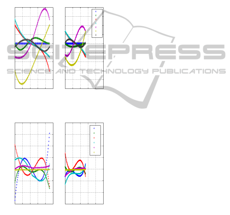
the amplitude of the leg angles is more important that
influences the maximum values of the torques so the
sthenic criterion is increased.
The fig. 7 presents the evolution of torques for the
walking speed of 0.2 m/s and confirms the previous
analysis. The torques of the robot are included be-
tween −3N.m and 3N.m for the B
´
ezier functions and
more than two for the cubic spline functions.
0 0.2 0.4 0.6 0.8 1
−0.25
−0.2
−0.15
−0.1
−0.05
0
0.05
0.1
0.15
0.2
Time [s]
Angles [rad]
Cubic Spline Function
0 0.2 0.4 0.6 0.8 1
−0.25
−0.2
−0.15
−0.1
−0.05
0
0.05
0.1
0.15
0.2
Time [s]
Angles [rad]
Bezier Function
q0
q5
q1
q2
q3
q4
q6
Figure 6: Evolution of absolute angles for the walking speed
at 0.2 m/s.
0 0.2 0.4 0.6 0.8 1
−6
−4
−2
0
2
4
6
8
Time [s]
Torques [N.m]
Cubic Spline Function
0 0.2 0.4 0.6 0.8 1
−6
−4
−2
0
2
4
6
8
Time [s]
Torques [N.m]
Bézier Functions
Γ
1
Γ
2
Γ
3
Γ
4
Γ
5
Γ
6
Figure 7: Evolution of torques for the walking speed at 0.2
m/s.
6 DISCUSSION
The improvement of the sthenic criterion at low
speeds with B
´
ezier functions is the main result in this
article The strategy to increase the range of travel
without recharging the batteries is to choose at low
speeds B
´
ezier trajectories and for fast speeds, to use
the trajectories defined by cubic spline functions. A
study about the sensitivity of the parameters will be
necessary to knowthe parameters influence. From our
point of view, the acceleration parameters of the cubic
spline functions are too sensitive for walking speeds
lower to 0.2 m/s.
To conclude, the model of the robot with rolling knee
has been introduced and we have proposed reference
trajectories for this type of anthropomorphic robot.
Our simulation program computes the joint torques
and the forces on the feet for different trajectory func-
tions. These trajectories are then parametrized to al-
low the resolution of the energetic optimization prob-
lem. Two types of trajectories are defined and the
optimization process shows that the B
´
ezier functions
give a significant criterion reduction at slow walking
speeds. These trajectories can be used like reference
trajectories for the control to starting up the gait of
the biped robot. The simulations shows that the cu-
bic spline functions are better adapted for gait speeds
greater than 0.25 m/s.
In future, other gaits can be explored such as Double
Support Phases (DSP) including foot rotation. The
influence of the radii r
1
and r
2
represents another in-
teresting challenge for this type of robot design.
ACKNOWLEDGEMENTS
The authors gratefully acknowledge the contribu-
tion of French National Research Agency under the
project number ANR-09-SEGI-011-R2A2.
REFERENCES
Banno, Y., Harata, Y., Taji, K., and Uno, Y. (2009). Optimal
trajectory design for parametric excitation walking. In
2009 IEEE/RSJ Int. Conf. on Intelligent Robots and
Systems, IROS 2009, pages 3202–3207.
Chestnutt, J., Lau, M., Cheung, G., Kuffner, J., Hodgins,
J., and Kanade, T. (2005). Footstep planning for the
honda asimo humanoid. In Proceedings - IEEE In-
ternational Conference on Robotics and Automation,
volume 2005, pages 629–634.
Chevallereau, C., Grizzle, J., and Shih, C.-L. (2009).
Asymptotically stable walking of a five-link under-
actuated 3-d bipedal robot. IEEE Transactions on
Robotics, 25(1):37–50.
Evrard, P., Gribovskaya, E., Calinon, S., Billard, A., and
Kheddar, A. (2009). Teaching physical collabora-
tive tasks: Object-lifting case study with a humanoid.
In 9th IEEE-RAS International Conference on Hu-
manoid Robots, HUMANOIDS09, pages 399–404.
GaitOptimizationofaRollingKneeBipedatLowWalkingSpeeds
213

Gini, G., Scarfogliero, U., and Folgheraiter, M. (2007).
Human-oriented biped robot design: Insights into the
development of a truly anthropomorphic leg. In Pro-
ceedings - IEEE International Conference on Robotics
and Automation, pages 2910–2915.
Grizzle, J., Abba, G., and Plestan, F. (2001). Asymptot-
ically stable walking for biped robots: Analysis via
systems with impulse effects. IEEE Transactions on
Automatic Control, 46(1):51–64.
Hamon, A. and Aoustin, Y. (2010). Cross four-bar linkage
for the knees of a planar bipedal robot. In 10th IEEE-
RAS International Conference on Humanoid Robots,
Humanoids 2010, pages 379–384.
Hobon, M., Lakbakbi Elyaaqoubi, N., and Abba, G. (2011).
Quasi Optimal Gait of a Biped Robot with a Rolling
Knee Kinematic. In IFAC 18th World Congress 2011,
pages 11580–11587, Milano, Italy.
Kajita, S., Kanehiro, F., Kaneko, K., Fujiwara, K., Harada,
K., Yokoi, K., and Hirukawa, H. (2003). Biped walk-
ing pattern generation by using preview control of
zero-moment point. In Proceedings - IEEE Interna-
tional Conference on Robotics and Automation, vol-
ume 2, pages 1620–1626.
Khalil, W. and Dombre, E. (2002). Modeling, identification
and control of robots. Bristol, PA.
Lagarias, J. C., Reeds, J. A., Wright, M. H., and Wright,
P. E. (1998). Convergence properties of the nelder-
mead simplex method in low dimensions. SIAM J.
Optim., 9:112–147.
Pfeiffer, F. and Glocker, C. (1996). Multibody Dynamics
with Unilateral Contacts. Wiley, New York.
Sabourin, C. and Bruneau, O. (2005). Robustness of the
dynamic walk of a biped robot subjected to disturb-
ing external forces by using cmac neural networks.
Robotics and Autonomous Systems, 51(2-3):81–89.
Scheint, M., Sobotka, M., and Buss, M. (2008). Compli-
ance in gait synthesis: Effects on energy and gait. In
2008 8th IEEE-RAS International Conference on Hu-
manoid Robots, Humanoids 2008, pages 259–264.
Spong, M. and Vidyasagar, M. (1991). Robot dynamics and
control. John Wiley and Sons, New-York.
Tlalolini, D., Chevallereau, C., and Aoustin, Y. (2011).
Human-like walking: Optimal motion of a bipedal
robot with toe-rotation motion. IEEE/ASME Trans-
actions on Mechatronics, 16(2):310–320.
Van Oort, G., Carloni, R., Borgerink, D., and Stramigioli,
S. (2011). An energy efficient knee locking mecha-
nism for a dynamically walking robot. In Proceedings
- IEEE International Conference on Robotics and Au-
tomation, pages 2003–2008.
Wang, T., Chevallereau, C., and Rengifo, C. F. (2012).
Walking and steering control for a 3d biped robot con-
sidering ground contact and stability. Robotics and
Autonomous Systems, 60(7):962–977.
Westervelt, E. R., Grizzle, J., and Koditschek, D. E. (2001).
Hybrid zero dynamics of planar biped walkers. IEEE
Transactions on Automatic Control, 48:42–56.
APPENDIX
Table 2: Parameters of HYDRO¨ıD Robot.
Body Length Masse Inertia Position
moment of CoM
[m] [kg] [kg.m
2
] [m]
Feet 0.678 0.001 sx =
L
p
0.207 0.013
l
p
0.072 sz =
h
p
0.064 0.032
Tibia 0.392 2.188 0.028 0.168
Thigh 0.392 5.025 0.066 0.168
Trunk 0.543 29.27 0.81 0.192
ICINCO2013-10thInternationalConferenceonInformaticsinControl,AutomationandRobotics
214
