Some Aspects of Autonomous Robot Navigation with Unscented

HybridSLAM

Amir Monjazeb

1

, Jurek Z. Sasiadek

1

and Dan Necsulescu

2

1

Department of Mechanical and Aerospace Engineering, Carleton University, 1125 Colonel By Drive, Ottawa, Canada

2

Department of Mechanical Engineering, Ottawa University, 161 Louis Pasteur, CBY A205, Ottawa, Canada

Keywords: Simultaneous Localization And Mapping (SLAM) Problem, EKF, FastSLAM, HybridSLAM, Unscented

HybridSLAM, Cluttered Environment, Double Loop Closing, Absolute Error.

Abstract: This paper addresses the linearization process of an autonomous mobile robot utilizing the second order

Sterling polynomial interpolation specifically used for Unscented HybridSLAM algorithm. It describes the

implementation of the linearization method to estimate the posterior mean and covariance of the system.

The major interest is to apply linearized equations for a simultaneous localization and mapping case in a

non-domestic environment with a random distribution of landmarks. Using computer simulations,

Unscented HybridSLAM and the associated theoretical interpolation is examined for a double-loop scenario

and the efficacy of the Unscented HybridSLAM is validated.

1 INTRODUCTION

The main task of a feature-based SLAM algorithm is

to estimate the path of the robot and map of the

environment as accurate as possible. There are many

methods in which the robot uses different sensors to

measure positions of landmarks as well as pose of

the robot (Williams et al., 2002). Sensor readings are

analyzed in these methods to extract data from the

active or passive features in the environment to

match it with a-priori known information in order to

determine the current position of the robot. Usually,

the task of extracting and matching data with a-

priori information is easy for a domestic

environment in which landmarks are distributed

evenly. If the robot has a notation of evenly

distribution of landmarks, the extracting of such data

would be rather easier. For some SLAM cases in

which the robot is equipped with restricted sensors, a

uniform distribution of landmarks would

considerably reduce the ambiguity of data

association in the environment (Sasiadek et al.,

2008). The advantage in such cases would be the

elimination of data extracted from wrongly observed

landmarks. Since the robot is aware of a uniform set

of landmarks, sensor readings that result more than a

specific threshold would be automatically deleted

from the estimation process as a result of the

Maximum Likelihood Rule (Thrun et al., 2004).

2 STERLING POLYNOMIAL

INTERPOLATION

The formulation of the second order Sterling

Polynomial Interpolation (SPI) is the basis of

derivation of the Divided Deference Filter (DDF)

and the Central Difference Filter (CDF) (Norgard et

al., 2000). To formulate the equations of the system

in a linear form, the second order SPI will be

discussed in this section to indicate how a non-linear

system can be approximated in a linear form. Then,

the mean and covariance of the system in the

posterior state will be discussed. Based on Taylor

series of a non-linear function in [5], a random

variable

x

around a statistical point

x

as its mean,

can be expressed by

 hDhDxhxh

xx

2

!2

1

)()(



2

)(

!2

1)(

)()(

dx

xhd

xx

dx

xdh

xxxh 

(1)

The SPI formula (Julier, Uhlmann, 2004) uses a

finite number of functional evaluations to

approximate the above non-linear function with

x

D



~

as the first and

2

~

x

D



as the second order central

divided difference operators acting on h(x),

 is the

interval length or central difference step size and

66

Monjazeb A., Z. Sasiadek J. and Necsulescu D..

Some Aspects of Autonomous Robot Navigation with Unscented HybridSLAM.

DOI: 10.5220/0004452700660073

In Proceedings of the 10th International Conference on Informatics in Control, Automation and Robotics (ICINCO-2013), pages 66-73

ISBN: 978-989-8565-71-6

Copyright

c

 2013 SCITEPRESS (Science and Technology Publications, Lda.)

x

is the prior mean of x around which the expansion

is done. The resulting formula can be expressed as

hD

~

!

hD

~

)x(h)x(h

x

2

1





(2)





2

)x(h)x(h

)xx(D

~

x







(3)

2

22

2



 )x(h)x(h)x(h

)xx(D

~

x







(4)

In some cases (Dahlquist and Bjorck, 1974), the SPI

formula can be interpreted as the Taylor series. If

this formula is extended to the multi dimensional

case, the function h(x) may be obtained by first

stochastically decoupling the prior random variable

x by the linear transformation as

xSy

1

x





(5)

)(h)(h)(h

~

xySy 

x

(6)

where

x

S

is called Cholesky factor (Smith, Self, and

Cheesman, 1974) of the covariance matrix P

x

of x

such that P

x

=S

x

S

T

x

. It should be noted that Taylor

series expansion of h(.) and

(.)

~

h

is identical if the

expected value of vector x is E[x] and the covariance

of the system is the expected value of P

x

=

E[

)( xx 

T

], the transformation stochastically

decouples variables in x so that the interval

components of

y becomes mutually uncorrelated.

P

y

= E[

)( yy 

T

] = I

(7)

Assuming that L is the dimension of x and y

with



i

y

i

)( yy 

as the i

th

component of

y



(i=

1, … , L),

i

e

is the i

th

unit vector,

i

d

is the partial

first order difference,

2

i

d

is the partial second order

difference, and

i

m

is the mean operator (Monjazeb

et al. , 2012). Therefore,

)(h

~

h

~

ii

L

i

y

yD





















dm

1

(8)

222

111

()()()

ijy

LLL

yi y yq jj qq

ijq

hh











 



D

y





dmdmd

(9)



)(h

~

)(h

~

)(h

~

iii

eyeyy 





2

1

d

(10)

2

1

() ( ) ( ) 2()

2

ii

hhh h







yyeyey

 





2

i

d

(11)



)(h

~

)(h

~

)(h

~

iii

eyeyy  

2

1

m

(12)

using equations (5) and (6) and considering that

i

x

s is the i

th

column of the Cholesky factor of

covariance matrix of x we can induce





ixi

hh eySey   ()(

~

)s()(

i

xixx

hh   xeSyS

(13)



i

x

s

ix

eS

= (

x

S

)

i

=(

x

P

)

i

(14)

Set of vectors defined in equation (13) is equivalent

so that that the UKF generates its set of sigma-points

with only the difference in the value of the

weighting term (Julier and Uhlmann, 2001).

3 POSTERIOR MEAN

AND COVARIANCE

ESTIMATION

The observation function can be expressed through a

non-linear function h(.) and with considering non-

linear transformation of an L dimensional random

variable x with covariance P

x

and mean x as follows

2

1

() () ()

2

kkkk

hhh h hzx y yD D

  



(15)

xSy

x



(16)

The posterior mean of

y

and its covariance and

cross covariance are defined as



k

z

E[

k

z ]

(17)



k

z

P

E[

)(

kk

zz



)(

kk

zz 

T

]

(18)



k

z

k

x

P

E[

)(

kk

xx



)(

kk

zz 

T

]

(19)

Assuming that





y

)( yy



is a zero-mean unity

variance random variable which is symmetric

(Norgard et al., 2000) as defined in equation (5), the

mean is approximated as



k

z E[

hhh

k

~

2

1

~

)(

~

2

DDy 

]

(20)

=

)(h

~

k

y

E[

h

~

2

1

D

]

(21)

=

)(h

~

k

y

E[



















)(h

~

)

ki

L

i

y

i

y

2

1

2

1

d



(22)

=

()

k

h



y



2

1

()()2()

2

L

ii

kk k

i

hh h



 



ye ye y

 





(23)

SomeAspectsofAutonomousRobotNavigationwithUnscentedHybridSLAM

67

=

2

()

k

L

h



y







2

1

()()

2

L

ii

kk

i

hh



 



y

e

y

e







(24)

By rewriting the posterior mean in terms of motion

vector (Brooks and Bailey, 2009) we will have

2

()

kk

L

h



zx







2

1

(s)(s)

2

ii

L

x

kk

i

hh







xy







(25)

Using the identity

k

z = E[

k

z ] = E[

k

z ] + )(h

k

x – )(h

k

x

= E[

k

z ] + )(h

k

x – E[ )(h

k

x ]

= )(h

k

x + E[

k

z – )(h

k

x ]

(26)

k

z

P = E[ )(

kk

zz  )(

kk

zz 

T

]

= E[

)( )(h

kk

xz  )( )(h

kk

xz 

T

]

–E[

)( )(h

kk

xz  ]E[ )( )(h

kk

xz  ]

T

= E[

)( )(h

~

kk

yz  )( )(h

~

kk

yz 

T

]

– E[

)( )(h

~

kk

yz 

] E[

)( )(h

~

kk

yz 

]

T

(27)

From equation (15), the second order approximation

of

h

~

h

~

)(h

~

kk

2

1

DDy-z 

can be substituted into

equation (27) and therefore,

k

z

P  E[(

2

1

2

hhDD



)

×(

2

1

2

hhDD



)

T

]

–E[(

2

1

2

hhDD



)]

×E[(

2

1

2

hhDD



)]

T

(28)



y

)( yy  is symmetric, therefore, all

resulting odd-order expected moments have zero

value. Since the number of terms in this calculation

grows rapidly with the dimension of y, the inclusion

of such terms leads the computation highly complex.

As a result all components of the resulting fourth

order term, E[

4

1

(

h

~

2

D

) (

h

~

2

D

)

T

], that contains

cross differences in the expansion of equation (28)

are discarded. The extra effort worthwhile is not

considered since it is not possible to capture all

fourth order moments (Monjazeb, Sasiadek, and

Necsulescu, 2011). The approximation of the

covariance and cross-covariance matrices are

expressed as below. For the details refer to (Norgard

et al., 2000).

In equation (30) the odd-order moment terms are

all zero since

)(

kk

yy



is symmetric. The optimal

setting of the central difference interval

parameter,

 , is dictated by the prior distribution of

xSy

1

x





. For Gaussian priors, the optimal value of

h is thus h =

3

. For more details see (Norgard et

al., 2000).

k

z

P



2

1

4

1

(s)(s)

ii

L

kx kx

i

hh







xx

×[

(s)(s)

ii

kx kx

hh



xx]

T

+

2

4

1

4





1

L

i





[

(s)(s)2()

ii

xx

kk k

hh h



xx x

×

[

(s)(s)2()

ii

kx kx k

hh hxx x

]

T

]

(29)

k

x

k

z



P E[ ()

kk

xx()

kk

zz

T

]



E[(

x

S ()

kk

yy[

2

1

2

hhDD



-E[

2

1

2

hD



] ]

T

] = E[(

x

S ()

kk

yy[ hD



]

T

]

+

1

2

E[(

x

S ()

kk

yy[

2

hD



]

T

]

–

1

2

E[(

x

S ()

kk

yy]× E[

1

2

hD



]

2

(30)

= E[(

x

S ()

kk

yy[

hD



]

T

]

(31)

=

1

2



1

[( ) ( )

i

L

x

ki ki

i

hh



 



sye ye





T

(32)

=

1

2



1

[( ) ( )

ii i

L

xkx kx

i

hh







sxs xs

T

(33)

4 SIMULATIONS AND RESULTS

4.1 Landmark Estimation Threshold

Figure 1-a shows a path in an environment with a

ICINCO2013-10thInternationalConferenceonInformaticsinControl,AutomationandRobotics

68

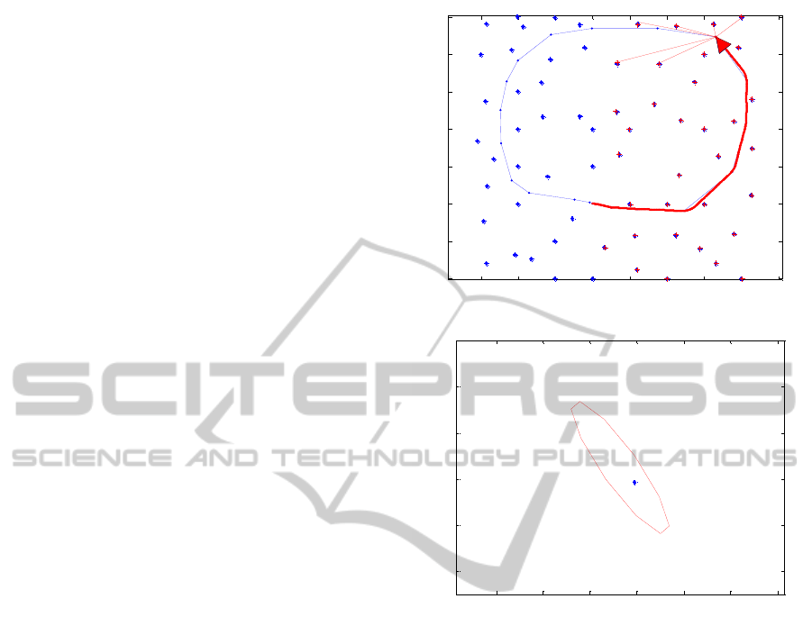
non-uniform distribution of landmarks. Figure 1-b

depicts the range of position estimation of landmark

at x=30m and y=20m. The error in this case

indicates that the estimated location of the landmark

is within ±0.40m. In this particular scenario, the

level of data ambiguity does not arise exponentially

when the distribution of landmarks change from

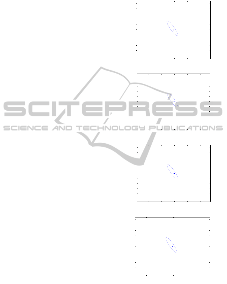
uniform to random. Figure 2 compares the

ambiguity of data with the use of EKF-SLAM as

well as using 3000 particles resulted by FastSLAM,

HybridSLAM, and Unscented HybridSLAM.

Hundreds of dots that make different formations

around in the range are depicted in this figure for

each specific algorithm. The threshold range (oval)

is obtained using a standard EKF under Gaussian

conditions. The true position of the landmark is at

x=30m and y=20m. The banana shape in figure 2-a,

shows the estimation result using the first order

Taylor series in EKF under non-Gaussian conditions

which appears to be highly inaccurate.

The banana shape in figure 2-b, illustrates a

reduction of error in the location estimation of the

landmark using FastSLAM and as a result less

ambiguity in data. However, estimated points do not

fit in the standard oval and there are about 60% of

estimated points off the standard threshold.

HybridSLAM has relatively less ambiguity in data

association as shown in figure 2-c. As shown in the

picture, there are only 30% of points outside the

range. Moreover, the estimation dots are mostly

inside the standard range. Nonetheless, it is still far

from the standard threshold and may not be an

acceptable result for SLAM applications. The

estimation of the landmark with Unscented Kalman

Filter creates an oval shape around the true location

of the landmark and is the one with the least

ambiguity in data association. As demonstrated in

figure 2-d, about 15% of estimated points are outside

the standard range which proves that HS has the

most acceptable result amongst all other algorithms.

As a result, UHS is the only algorithm which is a

recursive filter based on sterling approximation and

has the least tendency to diverge. Figures 3 to 5

demonstrate the performance of Unscented

HybridSLAM for the scenario depicted in figure 1.

In figure 5 the location estimation error of landmark

(x=10, y=0) is approximately 0.2m. In figure 6 the

error of location estimation of landmark (x=30,

y=40) is approximately 0.25m.

4.2 Double Loop Closing Scenario

In this section, simulation results of a double loop

-30 -20 -10 0 10 20 30 40 50

-20

-10

0

10

20

30

40

50

x direction

(

m

)

y direction (m)

Random Distribution of Landmarks

(a)

29.4 29.6 29.8 30 30.2 30.4 30.6

19.6

19.8

20

20.2

20.4

20.6

x direction (m)

y direction (m)

.

. .

.

. .

.

. .

.

. .

.

(b)

Figure 1: Random Distribution of Landmarks a) non-

uniform distribution of landmarks in the environment. b)

estimated position of the landmark located at (x=30,

y=20).

scenario using Unscented HybridSLAM algorithm

are presented. Here, the double loop closing case is

exemplified in order to analyze the performance of

the algorithm while the robot is travelling across

more complex terrain. Figure 7 shows a map of the

environment that contains an uneven distribution of

landmarks. The figure also shows the true path of

the robot. The speed of the mobile robot is assumed

3.5 m/s. The robot completes the whole loop in

approximately 2800 seconds. Number of particles

used in this experiment is 500. In figure 7 the true

map of the environment and observation results

before closing the loop are depicted. The vehicle

starts at the centre of the test area (x=0, y=0) and

travels counter clock wise. During the navigation

process landmarks are observed and the uncertainty

increases slightly. The uncertainty in the

SomeAspectsofAutonomousRobotNavigationwithUnscentedHybridSLAM

69

observations is at the largest value on the third part

of path. Figure 8 demonstrates the actual error and

standard deviations of the process when the robot is

at the third part of the path. Simulation results

illustrate the actual location error along x and y axes

respectively. Dashed lines represent the 1-sigma

estimated uncertainty. The simulated result indicates

that UHS is a consistent method with the actual

error.

Figure 9 shows the evolution of the uncertainty

for 4 out of 6 landmarks located in the smaller loop

at the beginning of the process. All solid lines

represent the deviations and dashed lines represent

the location estimation error. Comparing the error

between actual landmarks positions and those

estimated with the 2-sigma deviations indicate that

the UHS algorithm is consistent, specifically with

respect to landmarks location error. As expected, the

actual landmarks error and uncertainty have been

reduced. Two out of six landmarks were not

observed due to the scanner range limitations. Figure

10 shows the result in regard to the orientation

deviation and absolute error right after the loop is

closed and indicates that the map becomes more

correlated at the end of the first run. Figure 11

depicts the situation in which the loop is closed and

the robot is at one third of the path again. The robot

is at point (x=-20, y=34) and heading to complete

the second loop. The uncertainty in the observation

of landmarks at this point is considerably reduced,

meaning that the outcome of loop closing is

successful and the filter converges. Moreover, all

observable landmarks have been estimated correctly

following the completion of the first run. Figure 12

demonstrates absolute error and deviations along x

and y axes, the orientation, and for six landmarks

inside the internal loop after the robot completes the

loop and is at one third of its path during completion

of the second loop. The evolution of the uncertainty

for all six landmarks in the map indicate that the

map correlation in maintained and leads the final

map to be consistent. These results show that the

estimated uncertainty is consistent with the actual

error along both axes and the orientation of the

vehicle. The orientation error is around 0.02 radians

which confirms Unscented HybridSLAM algorithm

consistency.

29 29.5 30 30.5 31

19

19.2

19.4

19.6

19.8

20

20.2

20.4

20.6

20.8

21

x direction (m)

y direction (m)

.

. .

.

. .

.

. .

.

. .

.

. .

.

. .

.

. .

.

. .

.

. .

.

. . .

.

. .

.

. .

.

. .

.

. .

.

. .

.

. .

. . .

.

. . .

.

. .

.

. . .

.

. .

.

. . . .

.

. .

.

. .

.

(a)

29 29.5 30 30.5 31

19

19.2

19.4

19.6

19.8

20

20.2

20.4

20.6

20.8

21

x direction (m)

y direction (m)

.

. . . .

.

. .

.

. .

.

. .

.

. .

.

. .

.

. . .

.

. .

.

. .

.

. . .

.

. .

.

. .

.

. .

.

. . .

.

. .

.

. .

. . . . .

.

. .

.

. .

.

. .

.

. .

.

. .

.

. .

.

. .

.

. .

.

(b)

29 29.5 30 30.5 31

19

19.2

19.4

19.6

19.8

20

20.2

20.4

20.6

20.8

21

x direction (m)

y direction (m)

.

. . . .

.

. .

.

. .

.

. . .

.

. .

.

. .

.

. .

.

. . .

.

. . .

.

. .

.

. .

.

. .

.

. .

.

. .

.

. .

.

. .

.

. .

.

. .

.

. . . .

.

. .

.

. .

.

. .

.

(c)

29 29.5 30 30.5 31

19

19.2

19.4

19.6

19.8

20

20.2

20.4

20.6

20.8

21

x direction (m)

y direction (m)

.

. .

.

. . . .

.

. .

.

. .

.

. . .

.

. .

.

. .

.

. . .

.

. .

.

. .

.

. .

.

. .

.

. .

.

. .

.

. .

.

. . . .

.

. .

.

. .

.

. .

.

(d)

Figure 2: Estimated position of the landmarks a) EKF-

SLAM under non-Gaussian conditions b) FastSLAM c)

HybridSLAM d) Unscented HybridSLAM.

ICINCO2013-10thInternationalConferenceonInformaticsinControl,AutomationandRobotics

70

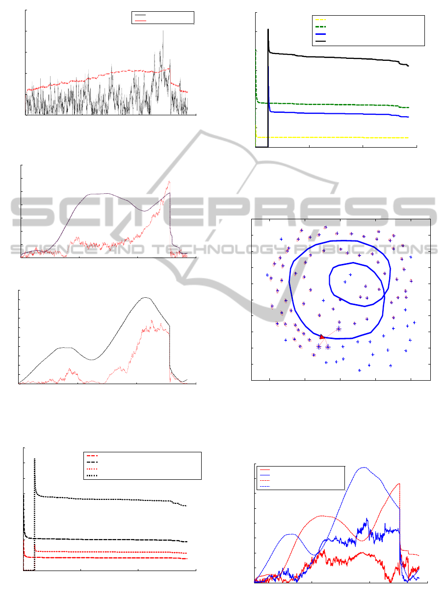
0 300 600 900

0

0.05

0.10

0.15

0.20

0.25

Absolute Error and deviation

Time (s)

Orientation (radi ans)

Absolute Error

Deviation

Figure 3: Orientation absolute error and deviation.

0 300 600 900

0

0.2

0.4

0.6

0.8

1

1.2

1.4

Time (s)

x di recti on (m)

Absolute Error and Deviation

(a)

0 300 600 900

0

0.2

0.4

0.6

0.8

1

1.2

1.4

1.6

1.8

2

Absolute Error and Deviation

Time (s)

y direction (m)

(b)

Figure 4: Deviation along a) x axis b) y axis.

0 50 100 150

0

0.2

0.4

0.6

0.8

1.0

1.2

1.4

1.6

Landmarks Deviation

Time (s)

Error (m)

Landmark (x=10 , y=0) Estimation

Landmark (x=10 , y=0) Deviation

Landmark (x=20 , y=0) Estimation

Landmark (x=20 , y=0) Deviation

Figure 5: Landmarks deviation (x=10 , y=0) and (x=20 ,

y=0) using 3000 particles.

750 800 850 900

0

0.1

0.2

0.3

0.4

0.5

0.6

0.7

Landmarks Deviation

Time (s)

Error (m)

Landmark (x=30 , y=40) Estimation

Landmark (x=30 , y=40) Deviation

Landmark (x=12 , y=48) Estimation

Landmark (x=12 , y=48) Deviation

Figure 6: landmarks deviation (x=30 , y=40) and (x=12 ,

y=48) using 3000 particles.

-50 -25 0 25 50

-50

-40

-30

-20

-10

0

10

20

30

40

50

y direction (m)

Before closing the loop

x direction (m)

Figure 7: True map of the environment with 94 observable

landmarks.

0 700 1400 2100

0

0.2

0.4

0.6

0.8

1

1.2

1.4

1.6

Absolute error and deviations along x and y axes

Time (s)

Erorr (m)

Absolute error in x direction

Absolute error in y direction

Deviation in x direction

Deviation in y direction

Figure 8: Absolute error and deviations.

SomeAspectsofAutonomousRobotNavigationwithUnscentedHybridSLAM

71

0 60 120 180

0

0.1

0.2

0.3

0.4

0.5

0.6

0.7

Time (s)

Error (m)

Landmarks Deviations and Absolute error

Figure 9: Landmark deviation and absolute error (a double

loop case) using 500 particles.

0 1000 2000 3000

0

0.02

0.04

0.06

0.08

0.10

0.12

0.14

Absolute Error and Deviation

Time (s)

Orientation (radians)

Orientatio n Error

Orientatio n Deviation

Figure 10: Orientation Absolute error and deviation

(double loop case) using 500 particles.

-50 -25 0 25 50

-50

-40

-30

-20

-10

0

10

20

30

40

50

x direction (m)

y direction (m)

After closing the loop

Figure 11: After the completion of the loop.

2800 2801 2802 2803 2804 2805 2806 2807 2808

0

0.05

0.10

0.15

0.20

0.25

0.30

0.40

Landmarks Deviation and Absolute error (at the begining of the second run)

Time (s)

Error (m)

Figure 12: Landmark deviation after closing the loop.

6 CONCLUSIONS

The major shortcoming of most simultaneous

localization and mapping algorithms is their

limitation to the first order accuracy of propagated

the mean and covariance as a result of first order

truncated Taylor series linearization technique.

Unscented HybridSLAM can address this issue with

the use of a deterministic sampling approach to

approximate the optimal gain and prediction terms in

a linear Bayesian form. Unscented HybridSLAM,

with its derivative-free Gaussian random variable

propagation technique, is able to calculate the

posterior mean and covariance of the system to the

second order of Taylor series. In order to show how

the model robot dynamics can be approximated, a

derivative-free technique based on Sterling’s

polynomial interpolation formula was derived and

presented in this paper. Derived equations were

linearized due to the high non-linearity of the

system. The second order Sterling Polynomial

Interpolation was employed to approximate a non-

linear function with first and second order central

divided difference operators acting on the

observation function expressed in a non-linear form.

Simulation results indicated that with the second

order Sterling polynomial linearization, Unscented

HybridSLAM gained enough accuracy and stability

in performance for double-loop scenarios in a non-

domestic environment.

REFERENCES

Williams, S. B., Dissanayake, G., Durrant-Whyte, H.,

2002, An Efficient Approach to the Simultaneous

ICINCO2013-10thInternationalConferenceonInformaticsinControl,AutomationandRobotics

72

Localisation and Mapping Problem”, Proceedings of

the 2002 IEEE International Conference on Robotics

& Automation, Washington DC.

Thrun, S., Montemerlo, M., Koller, D., Wegbreit, B.,

Nieto, J., Nebot, E., 2004, FastSLAM: an efficient

solution to the simultaneous localization and mapping

problem with unknown data association, Journal of

Machine Learning Research.

Norgard M., Poulsen N., Ravn O., 2000, Advances in

derivative-free state estimation for nonlinear systems,

Tech. Rep. IMM-REP, pp. 1998-2015, Dept. of

Modelling, Technical University of Denmark..

Julier, S. J., Uhlmann, J. K., 2004, Unscented filtering and

nonlinear estimation, Proc. of IEEE Journal, Vol. 92,

Issue 3, pp. 401-422, March.

Dahlquist G., Bjorck A. Numerical methods, 1974,

Prentice-Hall, NJ, Englewood Cliffs.

Smith R., Self M., Cheesman P., 1974, Estimating

uncertain spatial relationships in robotics,

Autonomous Robot Vehicles; Coxand & Wilforn Ed.,

Springer Verlag, pp. 167-193.

Monjazeb, A., Sasiadek, J. Z., Necsulescu, D., 2012,

Autonomous navigation of an outdoor mobile robot in

a cluttered environment using a combination of

unscented Kalman filter and a Rao-Blackwellised

particle filter, 2012, Proc. of 9

th

International

Conference on Informatics in Control Automation and

Robotics (ICINCO), pp. 485-488, Rome, Italy, July.

Monjazeb, A., Sasiadek, J. Z., Necsulescu, D., 2012, An

approach to autonomous navigation based on

Unscented HybridSLAM, Proc. of 17

th

International

Conference on Methods and Models in Automation

and Robotics, pp. 369-374, Miedzyzdroje, Poland.

Julier, S. J., Uhlmann, J. K., 2001, A counter example to

the theory of simultaneous localization and map

building, Proc. of IEEE International Conference on

Robotics and Automation, pp. 4238-4243, March.

Brooks, A., Bailey, T., 2009, HybridSLAM: Combining

FastSLAM and EKF-SLAM for reliable mapping,

Springer Tracts in Advanced Robotics, Volume 57, pp.

647-661.

Norgard M., Poulsen N., Ravn O., 2000, New

development in state estimation for nonlinear systems,

Journal of Automatica, pp. 1627-1638, Vol. 36, No.

11, November.

Monjazeb, A., Sasiadek, J. Z., Necsulescu, D.,

Autonomous navigation among large number of

nearby 2011, landmarks using FastSLAM and EKF-

SLAM; a comparative study, Proc. of 16

th

International Conference on Methods and Models in

Automation and Robotics (MMAR), pp. 369-374,

Miedzyzdroje, Poland.

Sasiadek, J. Z., Monjazeb, A., Necsulescu, D., 2008,

Navigation of an autonomous mobile robot using

EKF-SLAM and FastSLAM, Proc. of 16

th

Mediterranean Conference on Control and

Automation, pp. 517-522, Ajaccio, France.

SomeAspectsofAutonomousRobotNavigationwithUnscentedHybridSLAM

73