
Joint MAS-PDE Modeling of Forest Pest Insect
Dynamics: Analysis of the Bark Beetle’s Behavior
David Picard, Aymeric Histace and Marie-Charlotte Desseroit
ETIS UMR 8051, ENSEA, University of Cergy-Pontoise, CNRS, Cergy-Pontoise, France
Abstract. This article deals with the social behavior modeling of a particular
forest pest insect: the bark beetle. This ant-like insect has been responsible for
the devastation of acres of pines trees in North America since 2005. Any tactic
of forest pest management requiring prediction of pest population change over
time and/or space, a realistic modeling of beetle colonies behavior would be a
real benefit. The originality of this work is to propose a reactive Multi-Agent-
System integrating physical diffusion phenomena. The main idea is to take into
account the natural vanishing of the trail markers emitted both by decomposing
trees (ethanol) and the agents that have found a source of food (pheromone). The
proposed experiments show, on the one hand, that the MAS-PDE modeling leads
to a realistic global behavior of the colony when considering a usual foraging sce-
nario and, on the other hand, that, when compared with a simple reactive agent,
the proposed model has a faster convergence to the asymptotic usual expected
“S-shape” behavior of the agents’ colony.
1 Introduction
Modeling population dynamics is the essential part of both research and management
of forest pest insects. Any tactic of forest pest management requires prediction of pest
population change over time and/or space. However, the scope of prediction depends
on management objectives. An example of complex objective is to mi
nimize the impact of pest population on forest ecosystems during several years.
These kind of complex objectives require prediction of population changes over long
time intervals and over large areas. Of course, it is impossible to predict pest abundance
at specific location ten years ahead, but it may be possible to predict the change in
average pest population density as a result of some change in environment.
Formerly, to tackle this objective, mathematical modeling was the major tool for
predicting population dynamics and the reader could refer to Berryman and Millstein
[1] for a complete overview of some of the most known models that are mainly based
on modifications of discrete-time analog of the logistic model. The main advantage of
such methods is that parameters of these models can be adjusted to fit available data.
Nowadays, mathematical modeling based approaches tend to be replaced by Multi-
a
gent Modeling (MAM) that has constituted an important research and development
area for the past two decades [2]. A MAM is formed of two elements, a Multi-agent Sys-
tem (MAS), and an environment in which the MAS evolves. When designing a Multi-
agent model (MAM), the modeler has control over the multi-agent system behavior and
Picard D., Histace A. and Desseroit M..
Joint MAS-PDE Modeling of Forest Pest Insect Dynamics: Analysis of the Bark Beetle’s Behavior.
DOI: 10.5220/0004362100290038
In Proceedings of GEODIFF 2013 (GEODIFF-2013), pages 29-38
ISBN: 978-989-8565-49-5
Copyright
c
2013 SCITEPRESS (Science and Technology Publications, Lda.)

development and the environment. The latter is especially important in evolutionary
models as it determines the direction of the adaptation.
Fundamentally, a MAS is a system composed of multiple interacting agents within
an environment. The most simple MAS, called “reactive MAS” [3], assumes the behav-
ior of the agents can be modeled by a simple state machine (e.g. “resting”, “foraging”,
etc). These behavioral states often involve the modification of the environment (for in-
stance the deposit of a pheromone) or interacting with other agents. Such agents do not
have have any memory capability, nor any decision making process. Thus, the switch
from one behavior to another is performed in reaction to some changes of the environ-
ment or due to some interactions with other agents. However, the collective behavior
of the MAS, emerging from the interactions of the agents with the environment, can
often be far more complex than that of the agents alone. Ant colonies are a good start-
ing example for such MAS: Although the local behavior of a single ant does not seem
to be controlled centrally, nor any explicit coordination between ants is observable, the
superorganism “ant colony” is able to construct complex nest architectures or adapt its
distribution of foragers to food sources in an efficient way [4].
Cognitive MAS, based on a cognitive architecture, allows more complex behavior
modeling. A cognitive architecture can be defined as the organizational structure of
functional processes and knowledge representations that enable the modeling of cogni-
tive phenomena like memory [5]. Nevertheless, such MAS needs to have a very deep
knowledge about the individual behavior of each single agent of the colony, which is
not always easy to model when too few parametric data are available from the expert
(entomologists for instance).
Considering now the “environment” of the Multiagent Model [6], the related dy-
namic is usually considered as a static phenomenon. It means that a food source will
only be modified (location, quantity) by the interacting agents of the MAS but not
by possible underlying external physical phenomena (like diffusion for example). This
could be considered as a limitation since the environment has a strong influence onto
the global behavior of the agents.
The aim of this article is to propose a MAM based on a simple reactive MAS and
the taking into account of evolution physical laws related to the corresponding environ-
ment. More precisely, we want to show that by integrating the way the resources and
the trail markers could naturally vanish (steered by a diffusive phenomenon parametri-
cally described using the spatio-temporal heat equation), we can obtain a more realistic
modeling of the global behavior of the MAS dynamics.
Practically speaking, we focus our attention on the behavior modeling of an so-
cial pest insect: the “Bark beetle”. Bark beetles are ecologically and economically sig-
nificant [7] since outbreak species help to renew the forest by killing older trees and
other species aid in the decomposition of dead wood. However, several outbreak-prone
species are known as notorious pests that can cause tremendous damage to pine tree
forests for instance [8]. As a consequence, a better understanding of the social behavior
of this beetle would definitely be of some precious help to limit its damage capability.
This article is organized as follows: We first introduce the bark beetle species with a
focus on the entomological data. Second, we introduce the proposed MAM that permits
to model the social behavior of the bark beetle with a taking into account of the physical
30
law steering the inner evolution of the available resources in a given environment. We
then propose an experimental section in which the behavior of the model is shown.
Finally, the obtained modeling results are discussed and concluded.
2 A Social Pest Insect: The Bark Beetles
2.1 Bark Beetles Description
Bark beetles are so-named because the best known species reproduce in the inner bark
(living and dead phloem tissues) of trees. Some species, such as the mountain pine bee-
tle (Dendroctonus ponderosae), attack and kill live trees. Most, however,live in dead,
weakened, or dying hosts. Once beetles find a suitable host tree, they release aggregat-
ing pheromones to attract other beetles enabling a “mass attack” that can overwhelm
even a healthy tree defenses [7]. Along with releasing pheromones, the attacking bee-
tles introduce a staining fungus that infects and blocks the sapwood further weakening
the tree. Aggregating pheromones plus a pathogenic fungus infection help make rela-
tively healthy trees a quick meal for bark beetles.
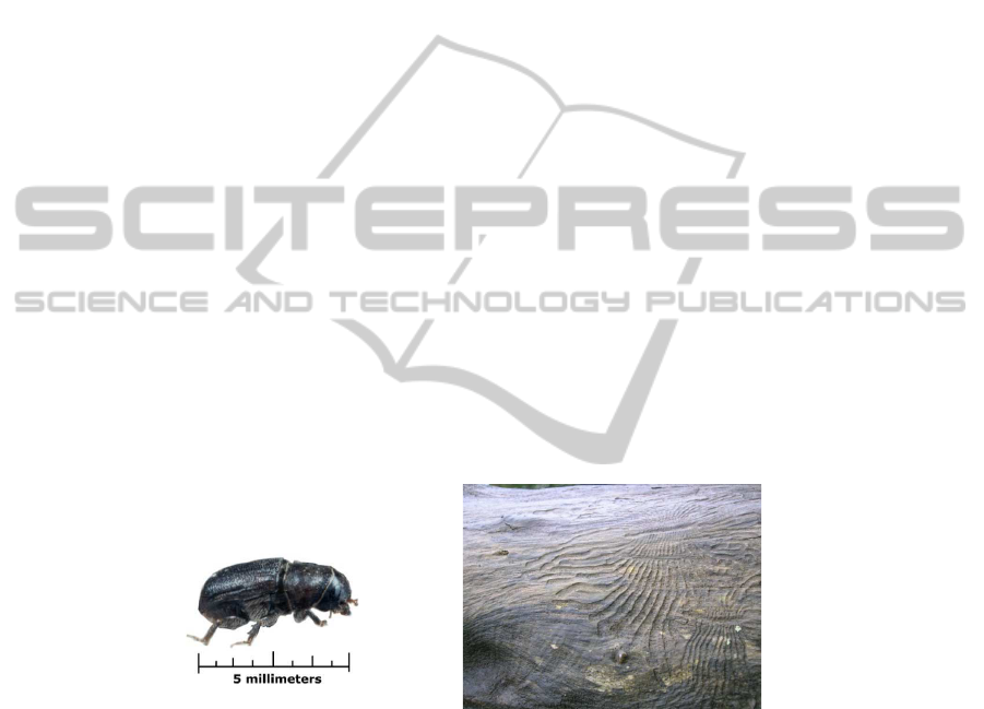
Most bark beetles look the same to the casual observer. Bark beetles are usually less
than 5mm long, shiny brown to black, cylindrical, with hard wing covers.Basically, they
look like everyday beetles, only smaller (see Fig. 1(a) for illustration). Beetles spend
almost their entire life beneath tree bark. After mating, an “egg gallery” is excavated by
the female beetle, sometimes with help from a male friend. Eggs, laid along the sides
of the gallery, hatch within a few weeks. The larvae feed on the nutritious inner bark of
the tree, pupate, and then emerge as an adult. The adult beetle only spends a few days
outside the bark flying to relocate to a new host.
(a) A typical bark beetle (b) Colony galleries on a dead tree
Fig.1.
Bark beetles excavate egg galleries like tiny tunnels in the live inner bark (Fig. 1(b)).
Engraver beetles score the sapwood, too. Larvae excavate “larval mines”. Bark beetle
galleries weaken the host tree and eventually kill it by girdling. Water and nutrient
transport in the live inner bark and in the outer edge of the sapwood are effectively
disrupted.
31

2.2 Ecological Role
Bark beetles and forests evolved together. In balanced forests, beetles have many bene-
ficial roles. The most important are:
– Beetles “thin” naturally overstocked forests. Beetle-induced thinning is often irreg-
ular and patchy contributing to forest diversity. Gaps encourage changes in vegeta-
tion and forest structure beneficial to wildlife.
– Beetles help recycle old forests. Beetles introduce wood decay fungi through the
bark where adults burrow into trees. Decay fungi help to rapidly decompose wood
and hasten nutrient recycling back into the soil.
– Beetle killed trees are a food source important to birds and other insect predators.
Snags provide roosting and nesting habitat.
However, due to peculiar warm climatic conditions, some deregulation could ap-
pear in the natural balance between forests and bark beetle population growing. As
a consequence, massive outbreaks of a specific species of bark beetles (the mountain
pine beetles) in western North America in 2005 have killed millions of acres of for-
est from New Mexico to British Columbia threatening increases in mudslides, forest
fires and other adverse effects. A similarly aggressive species in Europe is the spruce
ips typographus. Another tiny bark beetle, the coffee berry borer, Hypothenemus
hampei is a major pest on coffee plantations around the world.
3 Modeling of Bark Beetles Behavior
In this section we explain the notations used in the paper, along with the physical quan-
tities we model.
3.1 Hypotheses and Notations
Bark beetles are social insects and consequently, the global behavior of a nest can be
modeled by a simple reactive MAS based on simple interaction among the different
agents. Three main hypothesis will steer the behavior of each agent : (i) They look for
food sources (pine trees for example) ; (ii) Once a food source is detected the agent
emit a particular pheromone that will strengthen the related path (the “trail markers”),
and (iii) food sources emit on their surroundings an attractor element (trees in decom-
position emit ethanol that naturally attract xylophagus insects).
For the experiments, we consider a 2D area of evolution. Each site of this area are
located using their cartesian coordinates (x, y). The following related notations are used
to characterize resources and agents:
32

Resources
Let s(x, y) denotes a food source (trees):
– the corresponding evolution law of the available resources is noted R
s
(t),
– the corresponding evolution law of the ethanol emission is noted E
s
(t),
– and E(x, y, t) denotes the quantity of ethanol at the coordinates (x, y) and for a
given instant t.
Agents
Let a(x, y) denotes an agent at the location (x, y) of the area
– n
s
(t) denotes the number of agents on a given site s,
– q
a
(t), the probability for a given agent a to quit the colony, at instant t,
– and p
a
(x, y, t) the probability of an agent to move to location (x, y), at instant t.
Moreover, agents are mobile only if they are not on a resources site.
4 Experiments
For all the following experiments, we will consider a closed homogenous SMA. Only
beetles will interact (no other types of agents) and that the total amount of agents will
stay the same (50 agents) all along the different experiments (no phenomenon like
“birth” or “death” of agents will be taken into account).
For all experiments, we use the usual logistic law to model the evolution of the
resources on a site:
R
s
(t + 1) = R
s
(t) − αn
s
(t) (1)
with α a given value representing the mean consumption rate of an agent between
two iterations of the evolving process. This non-linear choice is motivated by the fact
that numbers of agents related to a resource is not a fixed value all along the process.
4.1 Agents Departure Modeling
In this first scenario, only one resource is considered and 50 agents are located on it. We
want to test the effect of resources exhaustion on the mobility of the agents. We propose
to model the probability of departure of an agent by the ration of available resources at
time t:
q
a
(t) = 1 −
R
s
(t)
R
s
(0)
(2)
No emission of ethanol is taken into account (i.e. E
s
(t) = 0) nor emission of
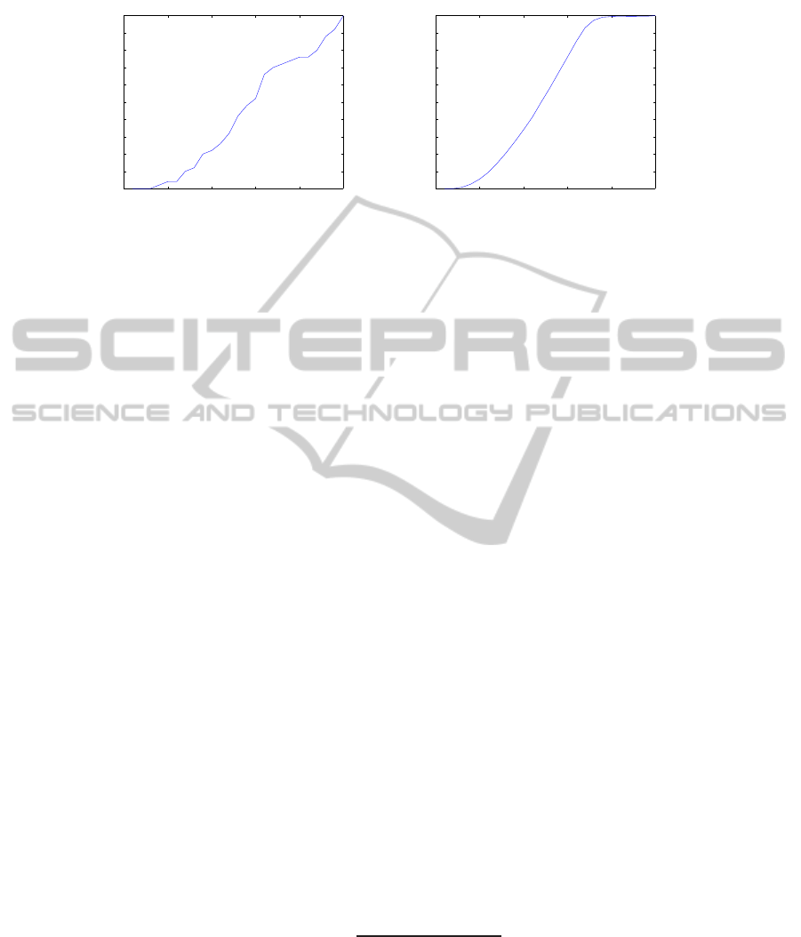
pheromone. Fig. 2.(a) shows the number of agents that turns to a “mobile” state against
the number of iterations.
A usual “S-phenomenon” [9] characterizes this evolution law. For a better illus-
tration, Fig.2.(b) shows the smoothed evolution law computed as a mean of the phe-
nomenon on 50 realizations. This first experiment shows the viability of our model
considering simple conditions of evolution. Let us know enrich the model.
33
0 5 10 15 20 25
0
5
10
15
20
25
30
35
40
45
50
(a)
0 5 10 15 20 25
0
5
10
15
20
25
30
35
40
45
50
(b)
Fig.2. Illustration of the “S-phenomenon” related to the number of “mobile” agents function of
the iteration number of the process for a unique resource site where all agents (50) are located at
t = 0: (a) for one realization of the experiment, (b) averaging on 50 realizations of the experi-
ments.
4.2 Resource Attraction and Aggregating Behavior Modeling
We now want to model the resources attraction phenomenon and the aggregating be-
havior of the agents. We consider the agents are randomly located all over the area of
evolution and that ethanol and pheromones are emitted respectively by the resource
sites and the agents which have found a resource site. The corresponding emission laws
are Gaussian functions such as:
E(x, y, t) =
X
s
E
s
(t)e
−γ[(x−x
s
)
2
+(y−y
s
)
2
]
, (3)
for ethanol emission (E
s
(t) = µR
s
(t), µ being a positive value lesser than one), and
P h(x, y, t) =
X
s
P h
s
(t)e
−γ[(x−x
s
)
2
+(y−y
s
)
2
]
, (4)
for pheromone emission (P h
s
(t) = νn
s
(t), ν being a positive value lesser than one).
We propose to model the probability of movement by the quantity of attracting
markers in the neighborhoodof the agents. Let us define the quantity of attracting mark-
ers A(x, y, t) as a coupling between ethanol and pheromones at location (x, y) and time
t:
A(x, y, t) = ηP h(x, y, t) + (1 − η)E
(
x, y, t) , (5)
with 0 ≤ η ≤ 1 being the coupling term. The probability to move to location
(x
⋆
, y
⋆
) for agent a is then:
p
a
(x
⋆
, y
⋆
) =
A(x
⋆
, y
⋆
, t)
X
(x,y)∈N (a)
A(x, y, t)
, (6)
34
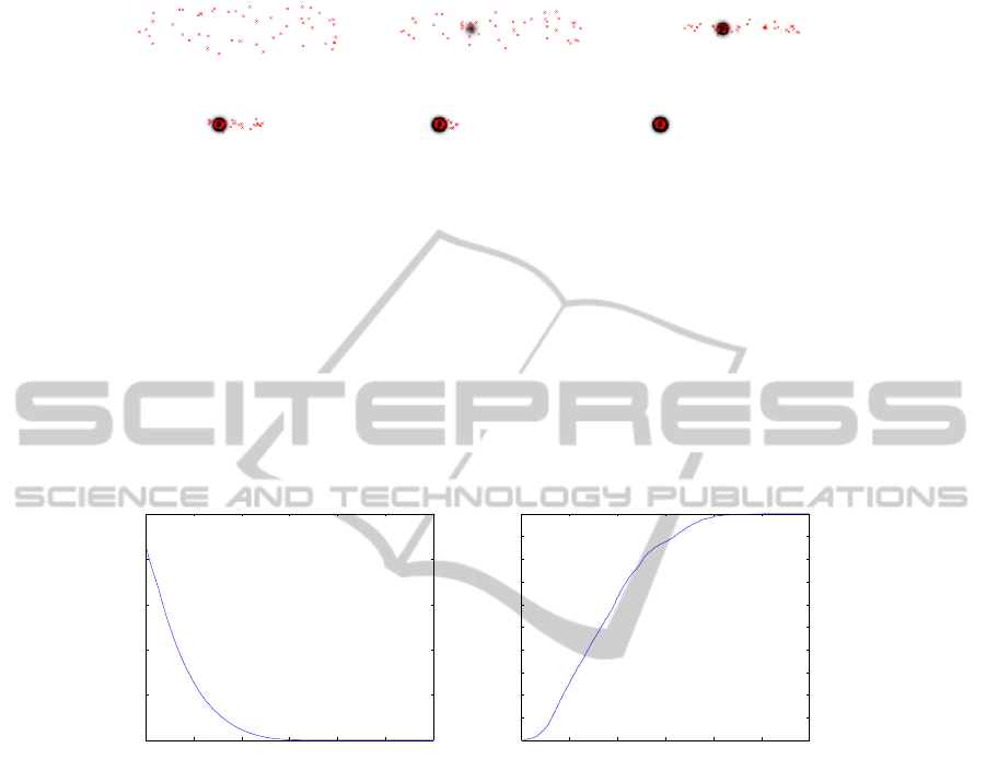
(a) (b) (c)
(d) (e) (f)
Fig.3. Illustration of Experiment 2: 50 agents are randomly dispatched all over the evolution area
(red stars) where a unique source of food is present. Evolution of the agents’ position is shown
for (a) iteration 0 of the process, (b) iteration 20, (c) iteration 60, (d) iteration 100, (e) iteration
140 and finally (f) iteration 180. The dark disk that progressively appears in the center of the
area highlights the position of the source of food, the gray level intensity is related to the level of
emitted pheromone: the more black, the more pheromone.
with N (a) being the neighborhood of agent a. In all our experiments, we consider 8-
connexity neighborhoods. Whenever an agent arrives on a resources site, it stops mov-
ing and starts emitting pheromones and consuming resources.
In Fig.3, we show the evolution of agents location as well as the pheromone levels
over time for a single run. As we can see, the agents are attracted to the resources site.
0 50 100 150 200 250 300
0
5
10
15
20
25
(a)
0 50 100 150 200 250 300
0
5
10
15
20
25
30
35
40
45
50
(b)
Fig.4. (a) Mean distance of the agents to the source of food function of the iteration number of
the process with η = 0.7. (b) Amount of agents on the source of food function of the iteration
number of the process (averaging on 50 realizations of the experiment)
In Fig. 4, we show (a) the mean distance of the bark beetles to the source of food
with η = 0.7 (more importance is given to pheromone emission than ethanol emission),
and (b) the amount of agents on the source of food over time t.
As we can see on Fig. 4.(a), the proposed model for ethanol and pheromone emis-
sion is compatible with a realistic modeling of the behavior of the beetles’ colony: for a
sufficient number of iterations (approximately 140) all the agents have converged to the
source of food. The exponential decreasing of the plot shows a two-step process: in a
first fast step, agents which are close from the resource site are attracted by the ethanol
emission of decomposing tree. Once they are on the resource site they then begin to
emit pheromone, attracting more and more agents. In a second step, due to the decreas-
ing of the resource, there’s a deceleration of the process since less and less ethanol is
35

emitted. Moreover, Fig. 4 .(b) shows the expected “S-phenomenon” related to that kind
of behavior.
Nevertheless, one limitation of this behavioral model is the insufficient taken into
account of the underlying physical phenomenonrelated to pheromone and ethanol emis-
sions. More precisely, if the Gaussian laws of Eqs. (3) and (4) are realistic, they do not
integrate any temporal dynamics highlighting for instance a natural diffusion process.
And yet, this diffusion scheme will interact with the attraction process by modifying the
expected p
a
probability. We now propose to integrate such a diffusive property within
the model.
5 Joint SMA-PDE Modeling
We now propose to consider that ethanol and pheromones are naturally dissipated
within the atmosphere at each iteration of the evolving process characterizing the colony
of beetles. For this, the simple isotropic diffusion process is considered. This physical
phenomenon is simple but as so, remains easy to control on the contrary of more com-
plex anisotropic processes. This natural phenomenon is mathematically defined by the
usual PDE of Eq. (7) also known as the “heat-equation”:
∂P h(x, y, t)
∂t
= △P h(x, y, t) =
∂
2
P h(x, y, t)
∂x
2
+
∂
2
P h(x, y, t)
∂y
2
(7)
with △, the Laplacian operator. If in Eq. (7), pheromone emission is considered, a
similar equation is related to natural diffusion of ethanol. Consequently, for each iter-
ation of the experiment, the initial distributions of pheromone and ethanol of Eqs. (3)
and (4) are naturally vanishing. Practically speaking, for each iteration t, Eqs. (3) and
(4) are convolved with a bidimensionnal Gaussian filter with standard deviation σ that
controls the speed of the isotropic diffusion. Iteration after iteration, the maximal am-
plitude of the pheromone emission is decreasing whereas the global spreading is made
over a larger surface of the area of simulation.
For the experiments, we set 2 different resources sites. At the beginning, all agents
are located on the first site, which has limited resources. On the contrary, the second
site has a near infinite quantity of resources. We expect the agents to quickly leave the
first site (as in section 4.1), and converge to the second site (as in section 4.2).
Fig. 5 shows the behavior of the beetles for different iteration of the process. As it
can be noticed, after a significant lapse of time corresponding to the random research
for food, the agents that are near the second site are attracted by the ethanol. Once these
agents find the resource site, the emission-diffusion of pheromone makes possible a fast
convergence of all agents to the corresponding site.
Fig. 6 shows the average distance of the agents from the initial point (x
0
, y
0
), func-
tion of the iteration number of the evolving process. The global behavior of the colony
is characterized by a double “S-phenomenon”. The first “S” corresponds to the small
pool of agents attracted by the ethanol at first, while the second “S” corresponds to
the remaining agents attracted by the pheromones. Compared to previous experiments,
the phenomenon is slower due to the initial location of the agents. Agents first exhaust
the food on their initial location, before they randomly move in the neighborhood. A
36
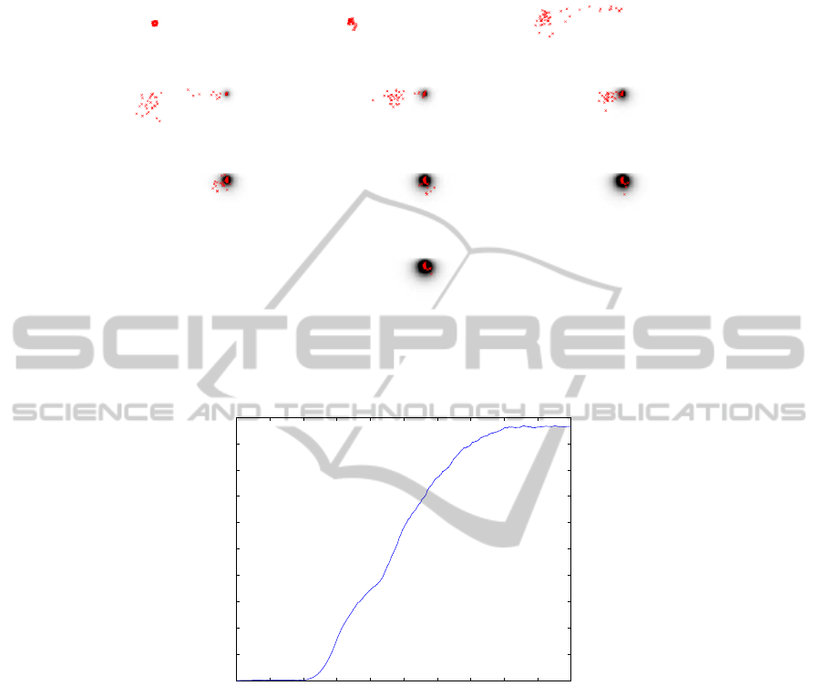
(a) t = 1 (b) t = 101 (c) t = 301
(d) t = 401 (e) t = 501 (f) t = 601
(g) t = 701 (h) t = 801 (i) t = 901
(j) t = 951
Fig.5. Beetles’ behavior corresponding to the joint SMA-PDA modeling proposed. σ is arbitrar-
ily set to 1.
0 100 200 300 400 500 600 700 800 900 1000
0
1000
2000
3000
4000
5000
6000
7000
8000
9000
10000
Fig.6. Average distance of the agents from the initial site they were localized at t = 0, function
of the iteration number of the process. Contrary to other experiments, this curve was obtained
with only one realization of the evolving process.
necessary significant lapse of time is needed for few agents to find the second source
thanks to the ethanol diffusion. Nevertheless, as soon as an agent is located on the new
resource site, the emission/diffusion of pheromone produces an acceleration of the con-
vergence when compared with experiment of section 4.2. Moreover, it is important to
notice that the “S-shape” of Fig. 6 was obtained with only one realization of the ex-
periment, whereas for Experiment 1 and 2, it was necessary to average the results over
50 realizations to obtain similar results. This shows the benefit of integrating the un-
derlying physical phenomenon that steers the natural evolution of pheromone/ethanol
diffusion, once emitted by agents.
37

6 Conclusions and Perspectives
In this article, a joint MAS-PDE for the modeling of the behavior of the bark beetle’s
colonies is presented. The main originality of the proposed approach is to integrate
within a simple reactive MAS some possible physical phenomena that steers the diffu-
sion of emitted substances like pheromone or ethanol. The prospective experiments of
this work show that such a joint model could lead to more realistic simulations of the
global behavior of the colony, with no need for multiple realizations of the process. If
this study is focused on the bark beetle, clearly identified since 2005 as a pest insect,
extensions to ant-like insects are straight forward. The next experiments will consist in
(i) improving the MAS by a managing of the “birth” and “death” of the beetles, but
also of the funding of new colonies by females, and(ii), in considering the possibility
to integrate more complex diffusion processes, like anisotropic ones, in order to take
into account the structure of the bark beetle’s nest within trees (galleries), and natural
perturbations like wind.
References
1. Berryman, A. A., Millstein, J. A.: Population analysis system. Pullman edn., Washington
(1994) Version 4.0.
2. Ferber, J.: Multi-Agent Systems: An Introduction to Distributed Artificial Intelligence.
Addison-Wesley (1999)
3. Demazeau, Y.: From interactions to collective behavior in agent-based systems. In: Proceed-
ings of the First European Conference on Cognitive Science. (1995) 117–132
4. Deneubourg, J., Goss, S.: Collective patterns and decision-making. 1 (1989) 295–311
5. Sun, R.: Cognitive Science Meets Multi-Agent Systems: A Prolegomenon. Phylosophical
Psychology 14 (2001) 5–28
6. Weyns, D., Parunak, H., Michel, F., Holvoet, T., Ferber, J.: Environments for Multiagent
Systems State-of-the-Art and Research Challenges. In: Proceedings of E4MAS. (2004) 1–47
7. Bentz, B.: Climate Change and Bark Beetles of the Western United States and Canada: Direct
and Indirect Effects. BioScience 8 (2010) 602–613 doi:10.1525/bio.2010.60.8.6.
8. Robins, J.: Bark Beetles Kill Millions of Acres of Trees in West. New York Times, 17
November (2008)
9. Langlois, P., Daud´e, E.: Concepts et mod´elisations de la diffusion g´eographique. Cybergeo:
European Journal of Geography 364 (2007) http://www.cybergeo.eu/index2898.html
38
