
Multi-protocol Scheduling for Service Provision in WSN
Michael Breza, Shusen Yang and Julie McCann
Department of Computing, Imperial College London, London, U.K.
Keywords:
Wireless Sensor Networks.
Abstract:
Currently, Wireless Sensor Network (WSN) systems are made of aggregates of different, non-related protocols
which often fail to function simultaneously. We present a self-organising solution that focuses on queue
length scheduling. To start, we define a network model and use it to prove that our solution is throughput
optimal. Then we evaluate it on two different WSN test-beds. Our results show that within the theoretical
communication capacity region of our WSN we outperform the current solutions by as much as 35%.
1 INTRODUCTION
Wireless sensor networks (WSNs) are networks of
small micro-controllers with sensors used to measure
phenomenon in the environment and then communi-
cate it via low-poweredradio. They are designed to be
diminutive in both physical size and acquisition price.
Small size enables their deployment in large numbers
and in a broad spectrum of inaccessible or dangerous
environments.
The capabilities of a WSN node vary depending
on the class of node; a shoe box size node is basically
a laptop, a matchbox size node has 16 MIPS micro-
controller with only hundreds of kilo-bytes of mem-
ory. It is the latter form of sensor network which is
the focus of this paper. Consequently the largest chal-
lenges involved in the development of WSN systems
are their limited resources. Typically they are battery
powered, so energy is a key constraint and the great-
est consumer of energy on a WSN node is the radio
transceiver. Radio communication is vital to trans-
form a group of sensor nodes into a coherent, usable
distributed sensing and computing system - where the
real power of WSNs lie.
In this work we focus on environmental monitor-
ing, a major application area for WSNs (Martinez
et al., 2006; Werner-Allen et al., ; Cardell-Oliver
et al., 2005). Environmental applications typically
have large numbers of sensors in different locations.
All the nodes sample environmental data at the same
time, and then send that data to a data collection
node(or base-station). The core WSN requirements
for this class of application is: time synchronisation,
dissemination of data to all of the nodes, and data col-
lection from the nodes. The current state of the art
in WSN system design, similar to general computing
systems, is that it uses separate protocols for each of
these functionalities. Protocols will share lower level
network stack information in order to optimise them-
selves (called cross-layer optimisation) but each pro-
tocol will have its own message type (or use multiple
message types) and therefore incur its own radio over-
head.
For example, the TinyOS (Levis et al., 2005) op-
erating system comes with a code library, which con-
tains many of the protocols used to enable the afore-
mentioned services. TinyOS protocols commonly
used for WSN are the Flooding Time Synchronisation
Protocol (FTSP) (Mar´oti et al., 2004) to synchronise
the sensor nodes and enable them to take time corre-
lated samples, the Deluge protocol (Hui and Culler,
2004) to disseminate updated code images to the en-
tire network, and the Collection Tree Protocol (CTP)
(Gnawali et al., 2009) to forward data collected by the
sensor nodes to a base-station for user processing.
Each protocol uses one or more message types,
and has their own communication requirement. As
we show, when combined, the summation of all of
the communication required by all protocols means
that collisions are likely and probable. Interference
can occur at the node level with one protocol starving
the other, and at the network level with nodes causing
radio communication failure for other nodes. This re-
sults in communication starvation for the service pro-
tocols causing the protocols to fail.
We are not the only researchers to notice this phe-
nomenon. Periodic heavy communicationrequired by
Deluge was shown to starve the Mint-Route data col-
14
Breza M., Yang S. and McCann J..
Multi-protocol Scheduling for Service Provision in WSN.
DOI: 10.5220/0004312800140022
In Proceedings of the 2nd International Conference on Sensor Networks (SENSORNETS-2013), pages 14-22
ISBN: 978-989-8565-45-7
Copyright
c
2013 SCITEPRESS (Science and Technology Publications, Lda.)

lection protocol off the beacons it needed to enable
data forwarding in (Hui and Culler, 2004; Langen-
doen et al., 2006). This caused the Mint-Route col-
lection protocol to fail, delivering only 2% of the data
sampled by the sensors. We have also observed the
same problem, where high data collection data rates
cause data dissemination to fail.
Two current approaches to solve this problem are
the Fair Waiting protocol (Choi et al., 2007) and the
Unified Broadcast layer (Hansen et al., 2011). The
Fair Waiting protocol is based on the notions of fair-
ness of channel usage. A scheduler keeps track of a
protocols usage, the more a protocol is used, the less it
gets scheduled. This mechanism was coupled with a
MAC layer back-off mechanism, where a node would
increase its medium access back-off time to reduce
the chance of collisions with other protocols. The
Unified Broadcast layer is a layer between the appli-
cation layer and the network layer where all broadcast
messages would be combined into one large message.
This layer handles the marshaling and marshaling of
the data and the delivery of the data to the correct pro-
tocol. It is transparent to the application layer proto-
cols.
Clearly, some form of system is required to man-
age these protocol services. The challenge of this sys-
tem is to maximise the use of the resources available
to it - within its capacity region. We begin by showing
the extent of the problem in section 2. Then our two
pronged approach to this problem is presented. At the
network layer we propose the use of a queue-length
scheduling scheme to maximise node resources which
we prove to be throughput optimal in section 3. We
evaluate our scheduler and show that they outperform
the current state of the art in sections 3.3 and 4. Fi-
nally we conclude in section 5.
2 THE EXTENT OF THE
PROBLEM
To understand multiple-protocol conflicts we devel-
oped a WSN temperature sensing application in our
laboratory. We used the state-of-the-art protocols pro-
vided in the TinyOS libraries so that the application
would be representative of the current standard way
to create a WSN application. The WSN consisted of
12 sensor nodes. The nodes sensed temperature and
sent this to a base station in a multi-hop fashion, see
Figure 1. We used CTP to collect data and route it to a
collection base station, and Deluge to disseminate up-
dated code images over the network. Both protocols
were chosen as they are the most popular for their pur-
3
0
1
2
4
5
6
7
8
9 10
11
12
Figure 1: Schema of laboratory with node placement and
desk locations.
pose. To create a baseline measurement, we observed
the percentage of data received by the base station us-
ing CTP in isolation. CTP worked well, averaging
99% data collection at a rate of 25 data messages re-
ceived at the base station every minute (the maximum
capacity stated in (Gnawali et al., 2009)). We also
ran the network with just Deluge. We found that Del-
uge performed very well, and that all the nodes were
updated and rebooted within a maximum time of one
minute.
We combined CTP and Deluge together and
looked at the same metrics: data collection rate (for
CTP), time to reboot, and percentage of the network
rebooted (updated by Deluge). Our first attempt was
with sampling and sending data once every minute.
Deluge updates were sent once every 30 minutes. The
data collection rate remained very high, around 99%,
but all of the Deluge updates failed to occur with in a
30 minute window. When this period was extended to
two hours, the updates still failed to occur. Reducing
the CTP data send rate to once every 10 minutes re-
sulted in a 99% success rate over a three hour period.
Deluge also worked, but took eight minutes and six
seconds for its first update and only succeeded in 10
out of 13 nodes used in the trial.
It is clear that when two protocols share the same
network stack, there is a chance of disruption occur-
ring to at least one of the protocols. This can be the
result of problems at one of two points in the network
stack, the MAC layer or the network layer. The MAC
layer may be unable to provide the protocols with the
bandwidth they need to function correctly. The net-
work layer may not be scheduling the protocols in
an efficient way, causing starvation to one or more
protocols. In either case one or more protocols may
not have the communication bandwidth which they
require to function properly.
Experiments were performed in order to test the
origin of the protocol failure we observed. To test
Multi-protocolSchedulingforServiceProvisioninWSN
15

the MAC layer, the number of collisions detected by
the radio were recorded. This was done by measur-
ing the CCA failures indicating the degree of network
congestion. Problems at the network layer were mea-
sured by recording the number of packets dropped by
the scheduling layer due to insufficient buffer space.
As results showed that there were no MAC layer
or scheduler problems during steady state CTP oper-
ation when there were no Deluge updates. When Del-
uge was used, both MAC layer and scheduler prob-
lems were observed. There were four times more
MAC layer collisions than messages dropped by the
scheduler. In the worst case the MAC layer indicated
11 failures while the scheduler had four lost packets.
More common results were four to six MAC layer er-
rors with one or two scheduler errors. Errors occurred
in 100% of the trials run with a data rate of a packet
every 20 seconds or more. Trials performed with a
data rate of less than 10 seconds failed to provide
the bandwidth needed for both protocols, and Deluge
failed to complete the dissemination of an entire code
image to any node. We conclude that a scheme that
both schedules the protocols and better shares net-
work medium is required.
2.1 Network and Channel Model
We model a one-hop WSN as a fully-connected, di-
rected graph G(N, L). The set of all sensor nodes
is N. All of the directional radio links between the
nodes is the set L. Time is divided into equal length,
non-overlapping time slots t = 1, 2, 3, ....
We denote the set of all of the protocols as P. Each
node maintains a message queue for each protocol in
P. The number of messages in a queue at node x ∈ N
for protocol p ∈ P at time slot t is Q
p
x
(t). All of the
queue message populations for all of the protocols on
all of the nodes is represented as the vector Q(t). This
vector can be seen as a matrix of |N| rows, one for
each node, and |P| columns, one for each protocol.
The value of each location in Q(t) our |N| × |P| ma-
trix is the corresponding number of messages in the
queue, Q
p
x
(t).
At time slot t, every protocol p ∈ P at every sen-
sor node x ∈ N adds messages to its queue with a rate
r
p
x
(t)(packets per slot). We assume that r
p
x
(t) is in-
dependent and identically distributed (i.i.d.) over all
time with a finite second moment where the expected
value of the square of the rate at which a protocol
adds to its message queue is less than the square of
the maximum finite message addition rate of all of the
protocols.
E[(r
p
x
(t))
2
] ≤ (r
max
)
2
. This assumption is safe for
environmental monitoring applications.
The rates at which each protocol adds messages to
its queues for all of the protocols on all of the nodes
is represented as the matrix r(t). This can be seen
as a matrix of |N| rows, one for each node, and |P|
columns, one for each protocol. The value of each
location in r(t) our matrix of size |N| × |P| is the
corresponding rate of message addition to the queue,
Q
p
x
(t).
2.2 Traffic and Data Queue Model
The rate at which a wireless link (x, y) ∈ L can for-
ward data, or send messages, at slot t is denoted as
c
x,y
(t). As our links are directional, this is only the
rate from node x to node y. The reverse rate may be
different. We assume that c
x,y
(t) is independent and
identically distributed (i.i.d.) over time (t), and with a
finite second moment E[(c
x,y
(t))
2
] ≤ (c
max
)
2
.
The broadcast capacity CB
x
(t) of a node x ∈ N is
the lowest rate c
x,y
(t) of all of that node’s links to its
neighbours.
CB
x
(t) = min
y∈N−{x}
c
x,y
(t), ∀x, y
The amount of data of a protocol p sent by a node
x in a time-slot t is f
p
x
(t).
This leads us to the intuitive conclusion that the
sum of all of the data sent by all of the protocols on
a single node must be less that or equal to that node’s
broadcast capacity
∑
p∈P
f
p
x
(t) ≤ CB
x
(t). The amount
a node sends in a time-slot can not exceed its capacity.
The queue length Q
p
x
(t + 1) is updated from time
period t to t + 1 by the equation:
Q
p
x
(t + 1) = max(0, r
p
x
(t) − f
p
x
(t) + Q
p
x
(t))
The queue length update equation is simply the
number of messages added in the previous time slot
minus the number of messages sent in that time slot,
added to the queue length at the start of that time slot.
To avoid message loss due to simultaneous trans-
mission of multiple nodes, only one node in N can
transmit during a time slot. This is because our local
area network G(N, L) is fully connected. Any other
nodes transmitting at that time will cause a collision.
Every node x has a contention-free transmission
vector with |N| dimensions called S
x
. Each value of
the vector corresponds to the CB
x
of a given node
x ∈ N for all nodes in the network, including the lo-
cal node. The x
th
entry of the vector is for node x
and is the broadcast capacity for that node. The vec-
tor S
x
itself represents only node x broadcasting at the
rate CB
x
and all of the other nodes remaining silent.
Therefore, the value of all of the other entries is zero.
SENSORNETS2013-2ndInternationalConferenceonSensorNetworks
16

The region Π is the convex hull over the |N| di-
mensional space of all of the contention-free trans-
mission vectors (S
x
). The space is defined as the re-
gion where all nodes can broadcast without causing
contention with one-another. The term a
x
is the long
term probability of the node x broadcasting.
Π = {S | S =
∑
x
a
x
S
x
, 0 ≤ a
x
≤ 1,
∑
x
a
x
= 1}
So, no combination of node sending schedules
which is outside of the space contained within the
convex envelope Π can be scheduled by any schedul-
ing policy. There will be contention and message loss.
2.3 The Network Capacity Region
The network capacity region is the set of all of the
rates at which all of the protocols can add new mes-
sages into their queues (r(t)) which can be scheduled
successfully. This means that the queue sizes will
not increase to infinity and that no messages will be
lost. Message loss due to overflowing queues is the
problem that we witnessed in our experiments above.
When the Deluge protocol began to send data it found
that the network capacity was not available to it, and
it failed.
The long term data broadcasting rate of a node x
is the sum of the long term data rates of all of its pro-
tocols p.
f
x
= lim
t→∞
1
T
∑
p∈P
T
∑
t=1
f
p
x
(t)
There is a vector f of size |N| which expresses the
average data rate required by every node in the net-
work. The value of the x
th
location in the vector is the
long term data rate of node x.
We formally define the network capacity region
as Λ and say that the data rates required by all of the
protocols are in the capacity region r ∈ Λ if there is a
scheduling algorithm which can provide the required
capacity.
f ∈ Π (1)
E[ f
p
x
(t)] ≥ E[r
d
x
(t)] ∀x ∈ N, p ∈ P (2)
These two conditions mean that as long as the re-
quirements of all of our protocols are in the capacity
region, then it is possible to schedule them, and en-
sure that the protocols queues do not overflow and we
do not lose messages. If the communication require-
ments of any of our protocols pushes our total data
rate f outside of the convex envelope of contention-
free schedules, then no scheduling policy will be able
to prevent message loss. If the protocol is not robust
to long term message loss and communication failure,
like we observed with Deluge when CTP was sending
at a high data rate, then the protocol will fail.
3 THE GREEDY QUEUES
SCHEDULER
The solution we propose follows from the analysis
above and combines medium access control and pro-
tocol scheduling. The protocol obtains each node’s
link quality between a node and all its neighbours to
maximise the chance of that message’s successful re-
ception by its neighbours. The queue length of the
different protocols wanting to use a node’s radio is
used to determine the next protocol to have radio ac-
cess.
At the beginning of every time slot t, every node x
identifies the protocol queue with the largest number
of messages p
∗
x
∈ P. It then uses that value and its
broadcast capacity CB
x
(t) to compute a weight w
x
(t).
w
x
(t) = CB
x
(t)max
p∈P
Q
p
x
(t) (3)
This weight is broadcast to all of a node’s neigh-
bours. When a node wants to broadcast a message,
it consults its table of node weights. If it is the node
with the highest weight x
∗
in the network at time slot
t, i.e. x
∗
= argmax
x∈N
w
x
(t) it will broadcast the next
data packet for protocol p
∗
x
. The short back-off cho-
sen by the node with the highest weight is less than the
minimum of the randomly chosen range of the initial
CSMA back-off to ensure that the chosen node com-
municates first.
f
p
x
(t) =
(
min(CB
x
(t), Q
p
x
(t)) if x = x
∗
, p = p
∗
x
∗
0 otherwise
(4)
If the node does not have the highest weight, then
it will use the normal random CSMA backoff time,
and send the next packet from the protocol with the
largest queue length p
∗
x
.
The Greedy Queue scheduler is a single-hop
scheduler. It is completely decentralised and uses
only local information. Each node makes a local deci-
sion how to act (when to communicate, and with what
protocol) based on local information and the informa-
tion of its local area neighbours. Next, we will prove
Multi-protocolSchedulingforServiceProvisioninWSN
17

our protocol is throughput optimal as long as the net-
work communication is within the network commu-
nication capacity.
3.1 Performance Analysis
This scheduling policy will ensure that the popula-
tions of all of the queues in the network do not exceed
their limits, and that no protocol has to drop packets.
This assurance can only be given as long as the data
sending rates of the nodes are within the channel ca-
pacity policy previously defined as r ∈ Λ.
Theorem 1. Given arriving traffic r such that r+ ε ∈
Λ for some ε > 0, our scheduling scheme will stabilise
the network.
Proof. To prove that our protocol queues will remain
bounded, we define the Lyapunov function:
V(t) =
∑
x∈N
∑
p∈P
(Q
p
x
(t))
2
(5)
Next, we consider its conditional expected drift:
E[△V(t)|Q(t)]
= E[V(t + 1)−V(t)|Q(t)]
= E[
∑
x∈N
∑
p∈P
((r
p
x
(t) − f
p
x
(t) + Q
p
x
(t))
2
− (Q
p
x
(t))
2
)|Q(t)]
≤ |N||P|(r
max
+ c
max
)
2
+2E[
∑
x∈N
∑
p∈P
(r
p
x
(t) − f
p
x
(t))Q
p
x
(t))|Q(t)]
≤
a
|N||P|(r
max
+ c
max
)
2
− 2ε[
∑
x∈N
∑
p∈P
Q
p
x
(t)|Q(t)]
The inequality ≤
a
, is because of (2) and our max-
weight scheduling scheme (4). Taking an expectation
over Q(t) and a telescopic sum from t = 1 to T, we
get:
E[V(T)] − E[V(1)] ≤ T|N||P|(r
max
+ c
max
)
2
−2ε
T
∑
t=1
(
∑
x∈N
∑
p∈P
E[Q
p
x
(t)])
Dividing both sides by T and taking an limsup we
see the long term expected queue length of each pro-
tocol on each node is less than or equal to a maximum
bound determined by the protocol’s message injection
rate and the proximity of that value to the edge of the
network capacity region.
limsup
T→∞
1
T
T
∑
t=1
∑
x∈N
∑
p∈P
E[Q
p
x
(t)] ≤
|N||P|(r
max
+ c
max
)
2
2ε
Then we see that as long as we remain in the ca-
pacity region, this bound is a finite number and there-
fore is less than infinity.
|N||P|(r
max
+ c
max
)
2
2ε
< ∞
This proof clearly shows that as long as the long
term rate at which all of the protocols on all of the
nodes inject messages into the network is in the ca-
pacity region, the long term expected value (or the
long term average) of all of queue lengths for all of the
protocols on all of the nodes will be less than or equal
to a finite value determined by the distance from the
message injection rate to the edge of the capacity re-
gion. This finite value is less than infinity. Therefore
proving that the Greedy Queues scheme is through-
put optimal within a given capacity region provided
by the system under consideration.
Please note that in our proof we use a limsup
but we could also just use a lim for two reasons.
Firstly, we assume environmental monitoring appli-
cations with a stable data rate. Secondly, we are only
concerned about the upper bound of the long term
data rate, not the lower bound, because the lower
bound will not cause our queues to overflow.
3.2 The Greedy Queues Scheduler
Implementation
We implemented the Greedy Queues Scheduler for
typical low power sensor nodes using TinyOS (Levis
et al., 2005) on the MicaZ and Telosb. The first mod-
ification to the default TinyOS networking stack is
to give each protocol a message queue. In the cur-
rent Active Message implementation, each protocol
gets its own queue with a length of one. This means
that if the protocol tries to send another message, it
receives an error message indicating that there is no
more buffer capacity. We lengthen the message queue
to 4 messages and implement it with FIFO semantics.
A queue depth of 4 messages was chosen for so as to
not consume too much memory. The second modifi-
cation we made was to include the weight defined in 3
in the broadcast message header. The weight is calcu-
lated using the packet reception ratio (PRR), that is,
the ratio of packets sent to a neighbours over pack-
ets received by that neighbour using the four bit link
estimator (Gnawali et al., 2009).
3.3 Single-hop Evaluation
Our aim is to enable the overlapping protocols to
function as best possible within the network’s com-
SENSORNETS2013-2ndInternationalConferenceonSensorNetworks
18
munication capacity region. To test the performance
of Greedy Queues we constructed a WSN running a
temperature sensing application. The sensor nodes
sense temperature and send data with a predefined fre-
quency to a base-station for logging.
We used a network of MicaZ motes with CC2420
radios. The transmission power level was set to full.
This gave us 0dBm of output power, and ensured that
all of the nodes in laboratory were connected to all
of the other nodes. The nodes had a minimum of
one meter distance between the aerials to prevent near
field radio interference. The size of the network was
varied from four nodes to 32 nodes.
We used FTSP for time synchronisation (Mar´oti
et al., 2004), Deluge to disseminate new code im-
ages (Hui and Culler, 2004), and CTP (Gnawali et al.,
2009) for data collection, to represent a typical envi-
ronmental monitoring application.
Protocol performance is application specific. For
Deluge it is the portion of the network that receives
and acts upon an update. We measured the time from
starting the dissemination, to the time the node re-
booted. For the data collection protocol, CTP, we
measure the percentage of sensor data packets deliv-
ered to the base-station. The results are an average
of 10 experimental runs lasting three hours each. The
data is taken from message log of data sent from the
base-station to a PC via serial port. For FTSP we mea-
sure the number of messages with synchronised time
stamps.
Temperature samples are sent to the base-station
every second. This data rate represents a heavy work
load. Once the network settles down and the col-
lection routes are established, Deluge is used to dis-
seminate a new code image throughout the network.
The code image consists of 38 pages, each page being
1024 bytes in size - the default page size for Deluge.
3.4 Single-hop Results
Since these experiments represent the search for a
scheduling policy which will allow multiple commu-
nication protocols to co-exist, it is important to take
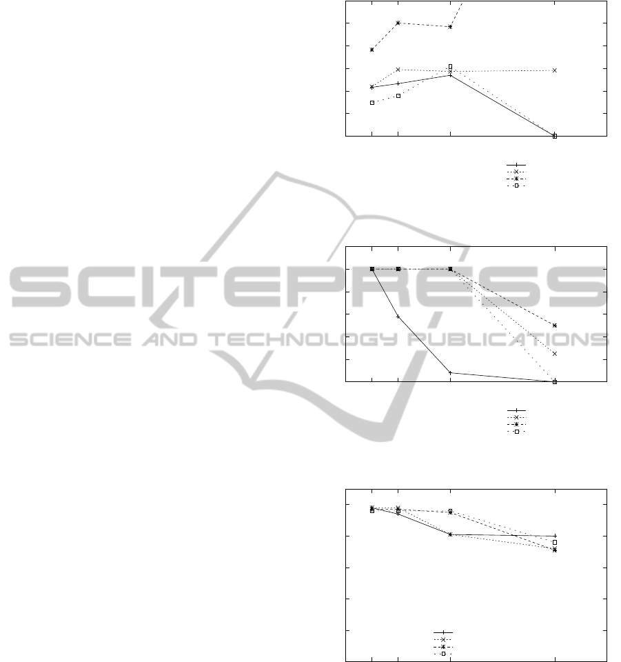
the three graphs together. The first graph (Figure 2)
shows the average time which the Deluge reprogram-
ming protocoltakes to reprogrammeour test-bed. The
times to disseminate need to be taken with graph (Fig-
ure 3) which shows how increasing neighbour pop-
ulation affects the percentage of successful dissemi-
nation trials for each scheduler. In cases where no
dissemination events were successful, the time to dis-
seminate drops to zero. When no dissemination was
successful, Deluge completely failed. The third graph
(Figure 4) shows CTP success rates as the network
Default Round Robin
Unified Broadcast
Fair Waiting Protocol
Greedy Queues
0
50
100
150
200
250
300
4 8 16 32
time in seconds
nodes in network
Figure 2: Plot of the time for each protocol to disseminate
an entire Deluge binary.
round robin
Unified Broadcast
Fair Waiting Protocol
Greedy Queues
0
20
40
60
80
100
120
4 8 16 32
Percentage of success
nodes in network
Figure 3: Plot of the percentage of trials where the Deluge
binary was successfully disseminated.
round robin
Unified Broadcast
Fair Waiting Protocol
Greedy Queues
0
20
40
60
80
100
4 8 16 32
Percentage of data received
nodes in network
Figure 4: Plot of the percentage of data message delivered
using CTP during the Deluge dissemination.
becomes congested and Deluge fails.
We see that Deluge works well with all of the
schedulers when the local neighbourhood population
is only four nodes. The time to disseminate is fairly
similar for all. The Fair Waiting Protocol works, but
is almost twice as slow as the others. The percent-
age of successful dissemination is 100% for all of the
scheduling policies, and all of the packets sent by the
Multi-protocolSchedulingforServiceProvisioninWSN
19

sensing nodes are received by the CTP base station.
These results give us a base case, where both proto-
cols run well as we are well within the capacity re-
gion.
When the population of the network is doubled to
eight nodes, the performance of the schedulers begin
to vary. The Unified Broadcast scheme hits an upper
bound for dissemination time at this point. In sub-
sequent trials its dissemination time remained fixed.
The time for FWP to disseminate increases to an av-
erage of 250 seconds, taking it off of the graph. The
Greedy Queues scheduler has the lowest dissemina-
tion time, 10% faster than the default Round Robin
scheduler. All protocols successfully complete 100%
of the Deluge trials except for the default Round
Robin scheduler. The percentage of data messages
received by the CTP base station is still very high for
all scheduler, in the 94% range.
The performance at a network population of 16
nodes is still good. The Deluge dissemination time
for all schedulers remains constant, or increases only
by a small amount. The percentage of Deluge trials
successfully completed is still 100% for all schedulers
except the default Round Robin scheduler, it succeeds
in only 5% of its trials. The percentage of CTP data
messages received by the base station remains con-
stant from the previous network populations for the
Greedy Queue scheduler and the Fair Waiting Proto-
col, and degrades by about 15% for the default Round
Robin scheduler and the Unified Broadcast layer.
At 32 nodes the phenomenon of protocol failure
becomes apparent. At this point the schemes are try-
ing to operate outside of the capacity region, as de-
fined in section 2.3, that is, beyond the constraints of
any scheduler. The time taken to disseminate Deluge
updates increase for the Fair Waiting Protocol to al-
most ten minutes, but only 50% of the disseminations
are successful as can be seen in Figure 3. Unified
Broadcast fared worse with about 30% success, tak-
ing the same time as for 16 and 8 nodes. The Greedy
Queue and the default Round Robin schedulers have
no successful dissemination attempts. In the case of
the Greedy Queue scheduler this was expected. The
throughput optimality of our scheduler is only defined
while the nodes send data at a rate which remains in
the capacity region.
The reception averages for CTP are for the most
part good. The Fair Waiting Protocol and Unified
Broadcast both manage about 70% data packet recep-
tion. The Greedy Queues protocol is more successful
and manage approximately 75% data reception.
In all cases the FTSP protocol functions properly.
This is because in a single-hop environment only the
FTSP synchronisation root will broadcast a sync bea-
con once every three seconds and therefore requires
very little communication overhead to function prop-
erly.
These results show us that we are able to cre-
ate a scheduling layer using only local information
to enable multiple protocols to function with good
performance at high data rates. As long as the rate
rates required by the protocols remains in the capac-
ity region, our greedy approach is able to use the
time previously lost to initial CSMA back-off periods,
and successfully schedule communication in that pe-
riod. The Greedy Queues scheduler shows the fastest
time to disseminate new Deluge code images. It also
maintains a data delivery rate equal to or better than
those of the other schedulers, even beyond the net-
work communication capacity region.
4 MULTI-HOP EVALUATION
The Greedy Queue scheduler was designed to opti-
mise local, single hop communication. We wanted
to see its effect on multi-hop communication scenar-
ios. For these experiments we decided to only evalu-
ate Greedy Queues against the default TinyOS round
robin scheduler. This is because the Fair Waiting Pro-
tocol only adds delays to reduce contention, and in a
multi-hop environment we found that the delays com-
pounded to make the system performance very slow.
The Unified Broadcast network layer did work very
well, but it worked by combining broadcast messages
and increasing the default message payload size from
28 bytes to 60 bytes to aim message combination and
reduce network traffic. This method is not a schedul-
ing approach, and therefore we do not compare our
scheduler against it.
4.1 In Laboratory Testbed
Our first multi-hop experiments used the same exper-
imental setup as for the one hop networks with 16
nodes. The radio transmission power was reduced to
power level 5 on the CC2420 radio used by the Mi-
caZ. This gave us about -20dBm of output power and
created a network with a maximum hop depth of 4
hops to the collection base station.
We used CTP to do data collection, and the nodes
sent at the rate of one data message every eighth of
a second. This rate was chosen by experimentation
to try and be as close to the edge of the capacity re-
gion of the network as possible. A separate Deluge
base-station was used to inject and disseminate new
code images into the network because it is difficult to
have one base-station handle both dissemination and
SENSORNETS2013-2ndInternationalConferenceonSensorNetworks
20

collection. Each code image was 38 pages, and each
page was 1024 bytes. The time was measured from
the time at which the deluge command was issued, to
the time at which the last node began its reboot. The
results are shown in Table 1.
We can see from this result that the average time
to disseminate is 43% faster with the Greedy Queues
scheduler than with the default TinyOS round robin
scheduler. Data collection is also improved by four
percent. In all cases the FTSP synchronisation proto-
col functioned properly. This experiment shows that
although the Greedy Queue scheduler only uses local
information to determine the protocol to send and the
backoff delay, it still provides benefits over the stan-
dard scheduler in a multi-hop network.
4.2 Remote Testbed
Our next set of experiments deployed the same set of
protocols on the remote wireless sensor testbed In-
driya (Doddavenkatappa et al., 2012). The testbed
contains 138 functioning nodes upon which these ex-
periments were run. This facility allows us to eval-
uate our protocol in a multi-hop environment, where
the population of the nodes is fixed. To vary load we
increased the sending rate of CTP, and then periodi-
cally disseminated large amounts of data using a Po-
lite broadcast dissemination protocol similar to Del-
uge. It was not possible to run the full Deluge proto-
col on the testbed because it does not allow the use of
the tosboot boot-loader. The boot-loader is used to re-
boot a node with a new code image, and is an integral
part of Deluge.
4.3 Multi-hop Evaluation
We can see in Figure 5 that as the rate of data sent by
each node (represented in Figure 5 as the number of
messages sent per second) decreases, the percentage
received by the base-station diminishes. When CTP
is on its own, not sharing the network with other pro-
tocols, its performance begins to degrade at the rate of
a data message sent every two seconds. At a message
every second, the base-station receives less than 45%
of the data messages sent.
The Greedy Queues and the round robin TinyOS
scheduler both have very similar performance to CTP
on its own up to the rate of one message every five
seconds. At a message every three seconds, both
scheduling policies lose the same percentage of data
messages. At higher data rates, the default Round
Robin scheduler loses on average 5% more mes-
sages that the Greedy Queue scheduler. The greedy
approach taken by our scheduler means that sensor
CTP only
Default Round Robin
Greedy Queues
0
20
40
60
80
100
0 2 4 6 8 10
Percentage of Received Messages
Percentage of Messages Received by CTP Basestation
Data messages sent per second
Figure 5: Percentage of data packets received by CTP per
data sending rate.
Default Round Robin
Greedy Queues
0
10
20
30
40
50
60
70
0 2 4 6 8 10
Seconds
Rate of data sending
Average Dissemination time per CTP data rate.
Figure 6: Average data dissemination times using Polite
Flooding.
nodes with the highest weight transmit with no delay,
and with a very low chance of interference. The re-
moval of the default CSMA back-off time allows us
to use the channel as efficiently as possible.
The data dissemination results in Figure 6 show
that under a heavy data communication load, the
Greedy Queue scheduler reduces dissemination time
by a minimum of 10%. The times are equal at lower
CTP data rates. At one message every three sec-
onds the dissemination messages start to get delayed.
One data message every two seconds shows that the
Greedy Queue scheduler has approximately 48% less
delay than the default Round Robin scheduler. By
the CTP data rate of one message every second, the
Greedy Queue scheduler is 35% percent faster than
the default Round Robin scheduler.
The synchronisation results are similar. The per-
centage of time 90% of network is in synchronised
state was higher for the Greedy Queue scheduler
across all data rates.
The Multi-hop evaluation results are similar to
those which we saw in the single-hop evaluation.
Once again the percentage of data packets received
Multi-protocolSchedulingforServiceProvisioninWSN
21

Table 1: The average percentage of data packets received by CTP.
dissemination time avg packets collected
Standard 431.5 sec. 80%
Greedy Queues 242.67 sec. 84%
at high data rates is better with the Greedy Queue
scheduler. Under the same conditions, the average
dissemination times are lower than for the default
Round Robin scheduler. These results show us that
as the network communication traffic increases, the
Greedy Queue scheduler can provide the network re-
quirements of each protocol better than the default
Round Robin scheduler currently in use.
5 CONCLUSIONS
Current environmental WSN systems are made by
combining several different protocols to provide the
services required by the application. This naive com-
bination can cause disruption or failure to one or more
of the protocols. Here, we propose a combined pro-
tocol and radio access scheduler which uses local in-
formation about protocol queue lengths and link ca-
pacities to enable multiple protocols to co-exist and
operate optimally within the network communication
capacity region.
We prove that our Greedy Queue scheduling
scheme is throughput optimal as long as the data rates
required by the protocols are within the capacity re-
gion of the network. Through evaluation we show that
it outperforms the current state of the art in a single-
hop network. We also demonstrate the same perfor-
mance gains in a multi-hop network. For future work
we would like to examine the affects of fairness on
the performance of the Greedy Queue scheduler.
REFERENCES
Cardell-Oliver, R., Kranz, M., Smettem, K., and Mayer, K.
(2005). A Reactive Soil Moisture Sensor Network:
Design and Field Evaluation. International Journal of
Distributed Sensor Networks, 1(2):149–162.
Choi, J., Lee, J., Chen, Z., and Levis, P. (2007). Fair waiting
protocol: achieving isolation in wireless sensornets.
In Proceedings of the 5th international conference on
Embedded networked sensor systems, pages 411–412.
ACM.
Doddavenkatappa, M., Chan, M., and Ananda, A. (2012).
Indriya: A low-cost, 3d wireless sensor network
testbed. Testbeds and Research Infrastructure. De-
velopment of Networks and Communities, pages 302–
316.
Gnawali, O., Fonseca, R., Jamieson, K., Moss, D., and
Levis, P. (2009). Collection tree protocol. In Proceed-
ings of the 7th ACM Conference on Embedded Net-
worked Sensor Systems, pages 1–14. ACM.
Hansen, M., Jurdak, R., and Kusy, B. (2011). Unified broad-
cast in sensor networks.
Hui, J. and Culler, D. (2004). The dynamic behavior of
a data dissemination protocol for network program-
ming at scale. In Proceedings of the 2nd international
conference on Embedded networked sensor systems,
pages 81–94. ACM.
Langendoen, K., Baggio, A., and Visser, O. (2006). Murphy
loves potatoes: Experiences from a pilot sensor net-
work deployment in precision agriculture. In Parallel
and Distributed Processing Symposium, 2006. IPDPS
2006. 20th International, pages 8–pp. IEEE.
Levis, P., Madden, S., Polastre, J., Szewczyk, R., White-
house, K., Woo, A., Gay, D., Hill, J., Welsh, M.,
Brewer, E., et al. (2005). TinyOS: An Operating Sys-
tem for Sensor Networks. Ambient Intelligence, pages
115–148.
Mar´oti, M., Kusy, B., Simon, G., and L´edeczi,
´
A. (2004).
The flooding time synchronization protocol. In
Proceedings of the 2nd international conference on
Embedded networked sensor systems, pages 39–49.
ACM.
Martinez, K., Padhy, P., Elsaify, A., Zou, G., Riddoch, A.,
Hart, J., and Ong, H. (2006). Deploying a Sensor Net-
work in an Extreme Environment. Sensor Networks,
Ubiquitous, and Trustworthy Computing, 2006. IEEE
International Conference on, 1.
Werner-Allen, G., Johnson, J., Ruiz, M., Lees, J., and
Welsh, M. Monitoring volcanic eruptions with a wire-
less sensor network. Wireless Sensor Networks, 2005.
Proceeedings of the Second European Workshop on,
pages 108–120.
SENSORNETS2013-2ndInternationalConferenceonSensorNetworks
22
