Detection and Classiﬁcation of Facades

Panagiotis Panagiotopoulos and Anastasios Delopoulos

Information Technologies Institute, Centre for Research and Technology Hellas, Thessaloniki, Greece

∗

Multimedia Understanding Group, Information Processing Lab, Department of Electrical and Computer Engineering,

Aristotle University of Thessaloniki, Thessaloniki, Greece

Keywords:

Facades, Probabilistic Modeling, Context-free Grammars, Recursion, Learning, Classiﬁcation, Window

Detection.

Abstract:

This paper presents a framework that exploits the expressive power of probabilistic geometric grammars to

cope with the task of facade classiﬁcation. In particular, we work on a dataset of rectiﬁed facades and we

attempt to discover the origin of a number of query facade segments, contaminated with noise. The building

block of our description are the windows of the facade. To this direction we develop an algorithm that achieves

to accurately detect them. Our core contribution though, lies on the probabilistic manipulation of the geometry

of the detected windows. In particular, we propose a simple probabilistic grammar to model this geometry and

we propose a methodology for learning the parameters of the grammar from a single instance of each facade

through a MAP estimation procedure. The produced generative model is essentially a detector of the particular

facade. After producing one model per facade in our dataset, we proceed with the classiﬁcation of the query

segments. Promising results indicate that the simultaneous use of an appearance model together with our

geometric formulation always achieved superior classiﬁcation rates than the exclusive use of the appearance

model itself, justifying the value of probabilistic geometric grammars for the task of facade classiﬁcation.

1 INTRODUCTION

Perhaps one of the most challenging problems in ma-

chine vision is the task of matching images of the

same object that have been photographed under dif-

ferent conditions (viewpoint, lighting conditions, oc-

clusions, etc). In this paper we present a methodology

that classiﬁes noisy query facade instances against

an original facade images. To this direction, we

construct a detector for each facade in our dataset,

i.e., a generative model that evaluates a query fa-

cade instance and we proceed to the classiﬁcation

task by evaluating all instances against all the de-

tectors. Since facades exhibit repetitive structures

and symmetries, it is not possible to directly apply

traditional matching techniques, like SIFT matching

(Lowe, 2004).

In this paper, we assume that a facade is gener-

ated from a context-free grammar with built-in ge-

ometric information, which uses elementary entities

(windows) as an alphabet. Such a grammar is called a

Probabilistic Geometric Grammar (PGG). In our set-

∗

This work was partially supported by the EU-funded

VITALAS project (FP6-045389)

ting, each grammar deﬁnes a generative facade model,

whose parameters are learned by a supervised, MAP

classiﬁer.

The idea of using grammars for object modeling

and recognition/detection is not new. In the litera-

ture, the study of syntactic pattern recognition was

pioneered by Fu et al (Fu, 1981; You and Fu, 1979).

In the mid 90’s, L-systems exploited the recursive na-

ture of grammars to model fractal structures, such as

plants and leaves (Holliday and Samal, 1995; Holli-

day and Samal, 1994). In particular, stochastic gram-

matical models were used in order to express the po-

tential uncertainty of the observed tree structures. Un-

like our approach however, L-systems did not model

the uncertainty of the produced geometry itself, as

each rule produced a particular geometry in a de-

terministic way. In recent years, more sophisticated

grammars, such as attribute graph grammars (Bau-

mann, 1995; Feng and Zhu, 2005; Zhu et al., 2010b;

Zhu et al., 2010a) and context sensitive graph gram-

mars (Rekers and Schurr, 1997) have been developed

to enable more powerful expressiveness and visual

inference mechanisms. Additionally, in the relevant

context of iterative and/or recursive patterns, there are

several approaches that examine the use of Frieze and

641

Panagiotopoulos P. and Delopoulos A..

Detection and Classiﬁcation of Facades.

DOI: 10.5220/0004283506410650

In Proceedings of the International Conference on Computer Vision Theory and Applications (VISAPP-2013), pages 641-650

ISBN: 978-989-8565-47-1

 2013 SCITEPRESS (Science and Technology Publications, Lda.)

Wallpaper groups for image modeling, matching or

Geo-tagging (Liu et al., 2004; Schindler et al., 2008).

However, they are not interested in the use of gram-

matical models. Finally, there is a number of recent

studies on the application of parsing facade images.

These studies use grammatical models for the proce-

dural modeling of buildings and facade reconstruction

(Muller et al., 2006; Wu et al., 2010; Wonka et al.,

2003; Ripperda and Brenner, 2009), or for scene in-

terpretation and segmentation (Teboul et al., 2011;

Teboul et al., 2010).

Intuitively, the use of grammars in facade classi-

ﬁcation is an attractive choice due to their ability to

describe compactly both the hierarchical and the re-

cursive structure of the particular objects. Although

there are several recent approaches that cope with the

task of image parsing of facades, we are not aware

of any approaches that proceed (after parsing) to their

classiﬁcation. To that direction, we propose a novel

approach that is capable of modeling both the struc-

tural and the geometric uncertainty of such structures

and evaluating images against these models.

Throughout this paper, we will use the grammar

of Table 1 to describe facades. The proposed gram-

mar describes facades as strings of entities that cor-

respond to speciﬁc parse trees. The leaf nodes of the

parse tree forming the string, i.e., the so called termi-

nal symbols, correspond to the visible substructures

of the facade, which in our case are the windows of

the building (symbol “w”). These structures are rep-

resented only by their 2D position in our analysis. On

the other hand, symbols “B” and “F” are the internal

nodes of the parse tree. These non-terminal symbols

correspond to the ﬂoors and the building itself. Their

position is not measured from the examined image.

In that sense we use the term invisible parts for non-

terminal symbols.

Perhaps the most important aspect in the deﬁni-

tion of our PGG is the inclusion of probability distri-

butions determining the relative position of the right

symbols of each replacement rule (children) with re-

spect to the left symbol (parent).

Our framework is essentially a part based model

(Felzenszwalb and Huttenlocher, 2005; Felzenszwalb

and Schwartz, 2007; Fergus et al., 2006). However,

the incorporation of grammars allows us to model fa-

cades whose size and structure may vary signiﬁcantly

among the various instantiations, due to the existence

of replacement rules that produce repetitions. More

importantly though and unlike traditional part-based

models, the use of grammars allows us to adopt a uni-

ﬁed description that models the original facade itself

and any other partial instance of the particular facade.

Which means that if we only see a part of a building,

the rest of it does not have to be considered occluded,

since it can be described by the adopted model. As

an additional note, although we do propose an ap-

pearance model in our experiments (Section 5), we

mainly focus on the ability of the grammatical model

to improve the classiﬁcation results when it is used to-

gether with this appearance model compared to the ef-

ﬁciency of the exclusive use of the appearance model

itself.

In Section 2, we present a formal representation

of PGGs and propose a modeling scheme that cap-

tures the statistical variance of positions. In Section 3

we formulate the bottom-up and top-down equations

that indicate how children nodes deﬁne the positions

of their parents and vice-versa. Based on these equa-

tions, we end up with closed-form expressions for es-

timating the parameters of our geometric distributions

and we propose a method for learning these param-

eters from a single image. In Section 4 we present

our window detection framework. Note that the over-

all methodology is not dependent on it since any al-

gorithm that accurately detects the positions of the

windows could be used instead. Section 5 presents

the classiﬁcation performance of the proposed frame-

work. Finally, conclusions are discussed in Section

2 PROBABILISTIC MODELING

2.1 Probabilistic Geometric Grammars

A PGG is a 5-tuple (V,Σ,R,S, F ), where V is a set

of symbols, Σ ⊂ V is the set of terminal symbols,

R ⊂ (V − Σ) ×V

∗

is a ﬁnite set of rules, S ∈ (V − Σ)

is the starting symbol and F is a set with f

k, j

∈ F

denoting the parameters of the generative geometric

model that produces the j-th child of the k-th rule.

It can be seen that PGGs are in essence context free

grammars (pages 113-120 in (Lewis and Papadim-

itriou, 1998)), including F .

According to the aforementioned deﬁnition, Table

1 shows the PGG that is used in this paper to describe

facades and Figure 1 displays a modeling example.

In this grammar, terminal symbols “w” express the

windows of the building and one can think of “F” as

representing the ﬂoors and “B” the building itself.

On the other hand, f

k, j

= {

k, j

,Σ

k, j

} are deﬁned

in Section 2.2 as the mean and covariance of a normal

distribution on the relative positions between a parent

node i and its j-th child in the parse tree, when pro-

duction rule r

is used.

Since PGGs are context free, the choice of a rule

does not affect the choice of other rules. Additionally,

VISAPP2013-InternationalConferenceonComputerVisionTheoryandApplications

642

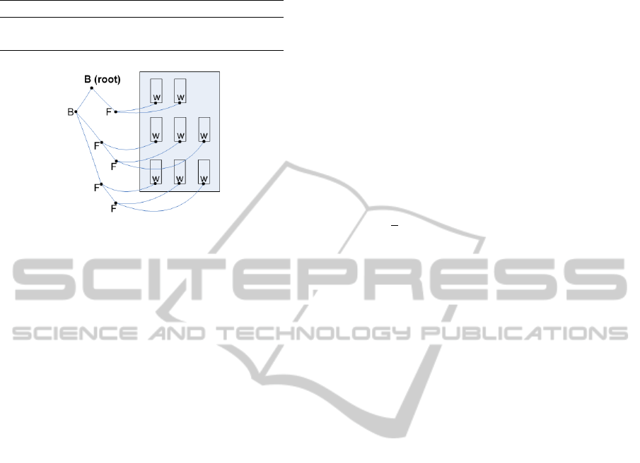
Table 1: A PGG for facades

V = {B, F,w}, Σ = {w}, S ≡ B, R = {r

,...,r

}

: B → BF r

: B → FF

: F → Fw r

: F → ww

Figure 1: A facade produced by the proposed grammar.

we assume that geometric relations among the chil-

dren of the same rule are independent to each other.

Geometric dependencies exist only among each child

and its parent. Since the employed grammar G in Ta-

ble 1 is in Chomsky Normal Form, let i index a non-

terminal node in a parse tree and ch

(i) and ch

(i) the

indices of the left and right child of i, respectively.

Moreover, let T be the set of all the parse trees of

this grammar and t ∈ T one of these parse trees. We

denote the probability of observing t, given that the

examined facade is some outcome of the grammar as

P(t|G). It can be interpreted as the probability of the

union of all the geometric relations in t. If we let

the relative position x

(i, j)

, j = 1,2 of node i with re-

spect to its j-th child represent the geometric relation

of these nodes, taking advantage of our independence

assumptions we can write:

P(t|G) =

∏

(i, j)

∈t

P(x

(i, j)

)

(1)

2.2 Probabilistic Modeling of Geometric

Relations x

(i, j)

Consider a rule r

from Table 1 and an instance of

this rule, consisting of a parent indexed as i and its

two children. We denote by y

the position of the par-

ent with respect to some global coordinate system and

(i)

and y

(i)

the corresponding absolute positions

of the two children. Then we consider:

(i, j)

= y

(i)

− y

(2)

as a random variable depending on y

Assume that we can measure the absolute posi-

tions of the two children of parent i, i.e., y

(i)

for

j = 1, 2. In order to estimate the position of the par-

ent, we would have to ﬁnd the MAP estimate of y

)

MAP

= argmax



|{y

(i)

}

j=1,2

o

= argmax



(i, j)

|{y

(i)

}

j=1,2

o

(3)

It is natural to let the probability on the right

hand side of Equation (3) follow a normal distribu-

tion. Since our grammar is context-free and we have

assumed statistical independence among the geomet-

ric relations of the children of the same rule (Equation

(1)), we can write:

P(x

(i, j)

(i)

) =

∏

j=1

P(x

(i, j)

(i)

)

∝ exp

(

−

∑

j=1

(i, j)

−

k, j

)

−1

k, j

(i, j)

−

k, j

)

(4)

where

k, j

and Σ

k, j

are the mean and the covariance

matrix of x

(i, j)

respectively, for all the instances i of

the rule k and for j = 1, 2.

3 GEOMETRIC DISTRIBUTION

PARAMETER ESTIMATION

Let us initially examine how to determine the posi-

tions of all the nodes in a parse tree, when the pa-

rameters of the normal distribution (means

k, j

and

covariances Σ

k, j

) are known. We identify two scenar-

ios. In the ﬁrst one, we are aware of the positions of

the children and we want to estimate recursively the

positions of the parent nodes (bottom-up). In the sec-

ond one, we know the position of a parent node and

we want to predict the positions of its children (top-

down).

Bottom-up Estimation. Consider two sibling

nodes produced by rule r

. If we knew the positions

of these two nodes and the values for

k, j

and Σ

k, j

where would their invisible parent be? In order to

ﬁnd the MAP estimate of the parent, we set the ﬁrst

derivative of Equation (4) with respect to y

equal to

zero, resulting to:

∑

j=1

−1

k, j

−1

∑

m=1

−1

k,m



(i)

−

k,m



, (5)

where

(i)

, for m = 1,2 denotes the previously es-

timated positions for the children.

Since we assumed that the statistical parameters

are known,

can be easily estimated. Moreover,

we can estimate all the non-terminal nodes by ap-

plying Equation 5 recursively from the leaves to the

DetectionandClassificationofFacades

643

root of the parse tree. In the special case that ch

(i)

for m = 1, 2 corresponds to leaf nodes, we make the

reasonable assumption that

(i)

≡ y

(i)

, so that

Equation 5 holds for all the nodes of the parse tree.

Equation (5) estimates a parent from its children and

thus, we call it bottom-up (BU) equation.

Top-down Prediction. Consider now the reverse

scenario where given the position of a parent node we

want to predict the positions of its children resulting

from replacement rule k. The predicted children po-

sitions are given by

(i)

k, j

, (6)

for j = 1, 2, where

is the measured or estimated

position of parent node i and

k, j

are the mean relative

positions of rule r

If we denote the position of the root node es-

timated by the BU equations as

, we can deﬁne

≡

, so that Equation 6 holds for the whole parse

tree. Applying Equation 6 recursively from the root to

the leaves, we can predict all the positions of the parse

tree. We shall refer to Equation (6) as the top-down

(TD) equation.

Throughout the rest of this paper, positions

marked with hats will be associated with BU esti-

mates, while positions marked with tildes will refer

to TD predictions. Moreover, we will employ the

two aforementioned notation assumptions that will be

used in order to proceed with the parameter estima-

tion, throughout Section 3.

3.1 Optimization Criteria

Consider a training set that consists of several parse

trees. Although we are aware of the structure of these

trees, we have no information regarding the position

of the non-terminal nodes. On the other hand we are

only able to measure the positions of the windows.

Our goal is to estimate the distribution parameters

(means

k, j

and covariances Σ

k, j

) of the generative

model.

Let us now examine Equation (5). We can see that

the position of the parent depends on the relation be-

tween the covariances of the children positions. Co-

variances on the other hand do not participate in TD

equations. Indeed, TD equations construct ideal trees,

based only on the mean values of the Gaussian dis-

tributions. Although we could try to discover a set

of parameters that would bring the TD and BU trees

as close as possible, this seems to be too demanding,

since the visible (and measurable) information is cap-

tured only on the leaves of the parse tree. Our genera-

tive model is in fact interested in producing accurately

only what is visible. Therefore, any set of parameters

that sufﬁciently explains the observed leaves of the

dataset can be accepted to be valid. We seek these

parameters that bring the estimated leaves as close as

possible to the observed ones. In order to achieve this,

we adopt the following optimality criterion:

Deﬁnition 1. The optimal means and covariances es-

timated are those that, if used in the BU procedure,

yield a parse tree root node that subsequently and via

the TD procedure generates leaf estimates that are as

close to the observed ones as possible.

In more detail, let our dataset consist of M fa-

cades or, equivalently, M parse trees. Each parse tree

t, t = 1,...,M has a number of m

leaf nodes, and

let P =

∑

t=1

be the total number of leaves. As-

sume an indexed collection I of all the nodes in the

dataset. Further assume that the indices of the leaf

nodes within I are i

, p = 1...P, so that all the leaf

nodes have absolute positions y

. If

Ψ = [(

1,1

,Σ

1,1

),(

1,2

,Σ

1,2

...,(

4,1

,Σ

4,1

),(

4,2

,Σ

4,2

)],

(7)

we seek:

Ψ = argmin

∑

p=1

−

(8)

For the sake of clarity, Table 2 introduces some

useful operators that will be used in the next sections.

3.2 Estimating Position Means

Consider a rule r

that produces one pair of terminal

nodes and let their parent be indexed with p. Since the

parent node is invisible, the only information we can

extract is the statistical behavior of one terminal node,

as observed from the other one, i.e, the quantity:

δY (p) = y

(p)

− y

(p)

(9)

We now seek these statistical parameters (

k,1

, Σ

k,1

k,2

,Σ

k,2

) that can reproduce the statistical behavior

of δY (p). Let’s focus on the covariance matrices; the

covariance of the positional difference of the children

will be:

= cov(y

(p)

− y

(p)

)

= cov(x

(p,1)

− x

(p,2)

) = C

(10)

where cov denotes the covariance and x

(p, j)

(p)

− y

) corresponds to the position of the par-

ent with respect to its j-th child. The last equation

holds because x

(p,1)

and x

(p,2)

are assumed indepen-

dent. Any pair of C

and C

that satisﬁes Equation

VISAPP2013-InternationalConferenceonComputerVisionTheoryandApplications

644

Table 2: Operators.

par(i

): index of the parent of node i

ind(i

): rule index and subindex of the rule that produced i

. If for example i

is the right child of

rule k, ind(i

) = [k, 2].

path(i

): all the indices of the nodes in the path from i

to the root (including i

and excluding the root).

term(d): indices of all the terminal nodes at depth d.

node(d): indices of all the nodes at depth d.

(10) is an acceptable choice for Σ

k,1

and Σ

k,2

respec-

tively. Therefore, we are free to choose:

k,1

= λC

k,2

= (1 − λ)C

(11)

with 0 < λ < 1.

This observation provides us with two important

beneﬁts:

1. We reduce the parameter space because we do not

have to estimate both covariances.

2. Equation (5) transforms to a covariance free ex-

pression. In the following, we choose λ = 0.5, so

that Equation (5) becomes:



(i)

−

k,1

(i)

−

k,2



(12)

It can be proved that using the same rationale, if

we denote with Σ

k,δy

the statistical covariance of the

positional differences of all the children produced by

rule k, we can generalize so that we can ﬁnd covari-

ances, such that:

k,1

k,2

= Σ

k,δy

/2 (13)

for all rules k = 1, ..., 4 that can produce the statistical

behavior of the observed leaves of a parse tree. We

adopt this choice and thus, in the sequel we shall use

Equation (12) instead of Equation (5).

In accordance to Deﬁnition 1, we will use the BU

and TD equations to ﬁnd an expression of the pre-

dicted leaf positions

, with respect to the measured

window positions y

and the mean positions of the

model. Consequently, we will estimate the position

means that minimize the distance between

and y

According to Equation (12), the position of the

root can be written as:

= 0.5

(0)

− 0.5

ind(ch

(0))

+ 0.5

(0)

− 0.5

ind(ch

(0))

By recursively eliminating the internal node posi-

tions, we come up with:

∑

d=1





∑

i∈term(d)

−

∑

j∈node(d)

ind( j)

(14)

where D is the maximum depth of the particular tree.

Equation (14) expresses the position of the root node

with respect to the measured window positions and

the mean positions.

In order to predict the position of the leaf node i

with respect to the position of the root node

, we

apply Equation (6) recursively, resulting to:

par(i

)

ind(i

)

par(par(i

))

ind(par(i

))

ind(i

)

= ···

∑

j∈path(i

)

ind( j)

(15)

The last equality in Equation (15) holds because, as

explained previously, the roots of the BU and the TD

trees are common so that

≡

Combining Equations (15) and (14) we can write:

− y

= M

X + c

(16)

so that

∑

d=1





∑

i∈term(d)

− y

, (17)

X = [

1,1

1,2

,··· ,

4,2

]

(18)

and



([1,1]),G

([1,2]),G

([2,1]),·· ·

··· , G

([4,2])



(19)

where

([a,b]) =

∑

j∈path(i

)

δ(ind( j) − [a,b])I

−

∑

d=1





∑

p∈node(d)

δ(ind(p) − [a,b])I

(20)

where I

is the 2 × 2 identity matrix and δ(A,B) = 1

iff A = B and 0 otherwise. Minimizing the L

norm of

Equation (16) for all the leaf nodes, we get:

∑

p=1





X +

∑

k=1





= 0 (21)

Equation (21) has a unique solution, so that:

X = −

∑

p=1





−1

∑

k=1





(22)

DetectionandClassificationofFacades

645

Matrix

∑

p=1





encodes the structure of

the parse trees and does not depend on the measured

positions of the leaf nodes. It is in general rank de-

ﬁcient. Regarding the employed grammar of Table

1, it is sufﬁcient to deﬁne one of the mean values on

each non-recursive rule (for example

2,1

and

4,1

Thus, we set arbitrary values the particular X entries

and solve for the remaining ones. The obtained solu-

tion, X

est

, is certainly a minimizer of Equation (8) and

hence, it describes the observations in the LSE sense.

3.3 Covariance Estimation

Since we have estimated the mean positions, we can

use the BU equations to estimate the positions of all

the internal nodes of the parse tree.

As explained before (Equation (13)), we assumed

that

k,1

k,2

= Σ

k,δy

/2, for all k = 1, ...,4 and all we

need is a way to estimate Σ

k,δy

. We proceed with the

estimation using the following procedure, for all the

rules in the grammar:

1. Pick a rule r

2. Identify all the instances of the particular rule in

the dataset, and let the corresponding parents be

indexed as k

...k

3. Estimate the sample mean of δY (k

), j = 1,...N

(Equation (9)), over the N instances of rule r

4. Estimate the sample covariance Σ

k,δy

δY (k

), j = 1,...N, over the N instances of

rule r

5. Choose:

k,1

k,2

= Σ

k,δy

/2.

3.4 Learning from a Single Image

Assume for a moment that we have achieved to detect

the windows of a facade and we have constructed its

parse tree (see Section 4). Since our ultimate goal is

to construct a detector for this facade, we are limited

to use a single image to produce the desired geometric

model. However, due to the employed grammar, the

second rule will appear only once in each facade. Ad-

ditionally, windows are not spread on a regular grid in

general, since the distance among windows may vary

across a building and we would like to capture this

behavior in the covariance matrices.

In order to to create a sufﬁcient dataset per facade,

we deﬁne a n × m segment as a part of the parse tree

that contains n ﬂoors and m windows per ﬂoor. We

construct a dataset that includes the original parsetree

and all the possible 3 × 3 parsetrees. If this is not

possible, in the case for example that n (or m) in the

original parse tree is 2, we set n (and/or m) equal to 2,

accordingly.

Conclusively, we learn one geometrical model per

facade, using the original parse tree and the selected

n × m segments, using the techniques described in

Section 3.

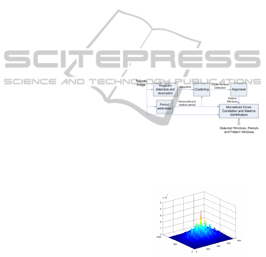
4 WINDOW DETECTION

The proposed window detection framework produces

the positions of the windows along with the horizontal

and vertical period and a set of characteristic windows

of each facade. Since we expect the detected windows

to lie on a grid, it is straightforward to deﬁne their or-

dering on the plane and therefore, the corresponding

parse tree (see also Figure 1). On the other hand, the

produced periods and characteristic windows of each

facade will be used for the detection of windows on

our test images, in Section 5.

Figure 2: The window detection diagram.

We initially approximate the horizontal and the

vertical period of each facade, namely T

and T

. This

is achieved by cross-correlating the image with itself

and calculating the distance between the two highest

consecutive peaks along each dimension (Figure 3).

Figure 3: Cross correlation of an image with itself. The dis-

tance between two consecutive peaks along each dimension

approximate the horizontal and vertical period.

In order to detect the windows we modify the

bottom-up approach described in the PhD thesis of

Olivier Teboul (Teboul, 2011). In particular we use

VISAPP2013-InternationalConferenceonComputerVisionTheoryandApplications

646

the FAST (Rosten et al., 2009) corner detector to de-

tect our interest points and we use the SIFT descriptor

with the same scale and orientation for all points.

From the large pool of the detected keypoints, we

have to determine which of them refer to windows and

choose one keypoint per window, for as many win-

dows as possible. This keypoint should describe the

same part of the window for every facade (a partic-

ular corner for example). To this direction, we uti-

lize a three step clustering scheme using the algorithm

proposed in (Komodakis et al., 2008). We justify the

choice of this algorithm for two reasons. First of all,

the number of clusters K is an output of the formula-

tion and in our case, K is unknown. Secondly, cluster

centers are necessarily members of the data set. We

use the L

norm as our distance function.

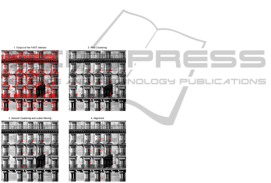
Figure 4: The ﬁrst clustering produces a number of clus-

ters, some of which refer to windows. We can see such a

cluster in the second image. In order to obtain one keypoint

per window, we perform the second clustering and we drop

potential outliers (third ﬁgure). We can see that in this case,

the outlier detection disposed several good windows. This

happened because this facade is not strictly periodic. The

windows on the left and right edges are further from their

neighbors, than the ones in the middle and T

expresses the

period in the middle windows. Finally in the fourth ﬁg-

ure, the detected windows are aligned. We can see that the

shaded window did not align very well. On the contrary,

the other window of the same ﬂoor moved to align with the

rest detected windows. The scope of this procedure is to

choose the patterns for the normalized cross correlation that

follows, in both the training and the testing phase.

First Clustering. In the ﬁrst clustering phase we

cluster the SIFT descriptors. The output of the ﬁrst

phase is a number of clusters, some of which do not

refer to windows. On the other hand, since it is natural

for neighboring keypoints that lie on the same edge to

have similar SIFT descriptors, clusters that do refer to

windows will have more than one keypoints per win-

dow, in general (see the second image of Figure 4).

Second Clustering. Our second clustering phase

aims at choosing exactly one keypoint per window.

We cluster the positions of the members of each clus-

ter from the ﬁrst clustering, so that windows are de-

scribed by the emerged cluster centers. We assume

that cluster centers should satisfy the estimated peri-

ods. Therefore, we examine each center and if there

are no other centers that lie in a horizontal (vertical)

distance close to T

), we consider the particular

center to be an outlier and we drop it (see the third

image of Figure 4). Although this is too strict and

we might drop points that lie on windows, we are still

interested to make a crude estimation that will be en-

hanced later.

Third Clustering. Our third clustering phase aims

at identifying which of the initial clusters refer to win-

dows. We separately cluster the horizontal and verti-

cal distance between all the pairs of cluster centers of

the second phase. For each dimension, if we discover

a cluster with respectable cardinality whose distance

is close to the corresponding period (T

and T

), we

consider that the cluster from the ﬁrst phase is refer-

ring to windows. For all the potential clusters that

refer to windows, we choose the one with the largest

cardinality.

Once we have chosen which of the initial clus-

ters we will use, we consider the corresponding clus-

ter centers from the second phase as an initial crude

estimation of some window positions. If we have

detected N windows, we choose N image segments

of T

× T

area, centered at the detected positions

,...,y

Alignment and Choise of Pattern Windows.

Since we want the window centers to represent the

same part of the window, we perform an iterative

alignment of the image segments. For each segment i,

we compute the normalized cross-correlation of i with

the rest j = 1,2, ..., i − 1, i + 1, ...,N segments. For

each one of the j segments, we locate the maximum

and we deviate y

towards y

, i.e.,y

= x

+ d(y

−

), where 0 < d < 1. We perform the same procedure

for 60 epochs until convergence. If some of the win-

dow centers fail to converge or fall out of the image

boundaries, we drop them. At the end of the align-

DetectionandClassificationofFacades

647

ment we have M windows of size T

× T

centered at

,...,y

. Let’s call them patterns.

Final Detection and Ordering of the Windows on

the plane. So far we have managed to detect some

windows in various locations of the facade and we

want to detect as many as possible. To this direc-

tion, we compute the normalized cross-correlation of

the original image with each one of the M patterns.

We aggregate the results using the max operator (Fig-

ure 5) and we search for the maxima that correspond

to windows. In particular, we assume that one of

the highest peaks is a window. If the coordinates

of this peak are [p

]

, we search for new win-

dows in an area of T

× T

, around [p

± T

]

and

± T

]

. The maxima within each one of these

four areas are our new windows. We continue the

same procedure recursively, making sure that we do

not search twice within the same area. The output of

this procedure is our ﬁnal choice of windows (Figure

6), along with their ordering. The order of windows is

deﬁned by the progress of window searching. If, for

example, we detect the i-th window of the j-th ﬂoor

at position [p

]

and then we manage to detect

another window in the area around [p

]

, the

new window will be the i+1 window of the j-th ﬂoor.

If on the other hand the new window is detected in the

area around [p

− T

]

, the new window will be

the i-th window of the j − 1 ﬂoor.

Figure 5: Cross Correlation of the original image with the

patterns. The peaks indicate the positions of the windows.

By examining the ordering, we can argue if this

procedure has missed any windows. There are two

cases of occlusion. In the ﬁrst case we identify gaps

in the ordering. For example if the ordering for one

ﬂoor is [1 2 4 5], we assume that the third window is

missing. In the second case, there are ﬂoors that have

less windows than the maximum number of windows

per ﬂoor, or the ﬁrst window of a ﬂoor is missing.

In the ﬁrst case we interpolate the missing windows

between the previous and the next detected ones. In

the second case, we extrapolate the missing windows

from the last or the ﬁrst detected window of the ﬂoor

that exhibits the occlusion, according to T

Figure 6: The ﬁnal detected windows.

5 RESULTS

We apply our approach on the Ecole Centrale Paris

Facades Database (Teboul, 2012) produced and

maintained by Olivier Teboul. In particular we focus

on the Paris, France collection of 215 rectiﬁed im-

ages. From each one of these images we crop a small

segment and our main goal is to discover the origin

of a distorted version of each segment wrt the original

215 images. Therefore, we want to compute 215 geo-

metric models and evaluate each test segment against

all models.

In order to compute these models, for each facade

we apply the window detection techniques described

in Section 4, we produce the parse trees (along with

the horizontal and vertical periods and the pattern

windows) and we learn the parameters, as described

in Section 3.

Then for each one of the cropped test segments

we follow similar steps as in the window detection

phase; we evaluate the normalized cross correlation

of the segment with each of the M patterns of the par-

ticular model, we aggregate using the max operator

and we search for windows using the periods T

and

that were estimated for the production of the partic-

ular model. Therefore we detect some windows and

their ordering and we produce the parse tree.

We proceed by utilizing an appearance model. In

particular, when our searching algorithm detects a

window, we crop a T

× T

area centered at the detec-

tion point and we compare it with the pattern window

that gave the maximum cross-correlation value at the

particular position. Let M

be the number of the de-

tected windows in the segment. We compute the mean

squared error S

between all the pixels of the j-th de-

tected window and the corresponding pattern and we

deﬁne the appearance likelihood of the image to be:

VISAPP2013-InternationalConferenceonComputerVisionTheoryandApplications

648

∑

i=1

. (23)

In order to estimate the geometric likelihood, we

estimate the frames of the non-terminal nodes using

the BU equations and we would normally use Equa-

tion (1). However, geometric likelihood is a decreas-

ing function of the size of the parse tree. In order to

compensate the fact that different models detect dif-

ferent number of windows, we evaluate the geometric

likelihood as:

logP(t|G)

, (24)

where P(t|G) is evaluated from Equation (1).

The overall expression of the likelihood is

P = P

− kP

, (25)

where k is a normalizing factor.

We perform the evaluation 25 times by grad-

ually blurring and adding noise to the segments.

In particular we use a Gaussian kernel with σ

0.8,1.3,1.8,2.3, 2.8 to blur the images and we add

random noise from a uniform distribution in [0,N],

where N = 90,130,170,210,250. With reference to

Figure 7, the original segment is blurred with the

Gaussian ﬁlter H

whose variance is σ

. The ran-

dom noise is initially ﬁltered with a Gaussian ﬁlter

whose variance is 1. We normalize the ﬁltered

noise by subtracting its mean value and we add it to

the blurred segment.

Figure 7: Blurring and adding noise to the original image

segments

Figure 8: The original test image and three noisy instances.

For each one of the 25 noise scenarios, we com-

pute the number of correct classiﬁcations and the

mean reciprocal rank (MRR) (Voorhees, 1999) for

two cases. In the ﬁrst one, we use only the appear-

ance model and in the second one we use both the

appearance and the geometric model. If there is no

noise present, our appearance model manages to clas-

sify all the samples correctly, making the use of our

geometric model unnecessary. However, we can see

in ﬁgures 9 and 10 that the contribution of the geomet-

ric model becomes signiﬁcant, as the noise increases.

The less our appearance model achieves to discover

the correct classiﬁcation, the more our geometrical

model contributes to the overall performance. As a

ﬁnal remark, we can see that the surfaces that repre-

sent the combined use of both models are constantly

above the surfaces that represent the explicit use of

the appearance model.

0.5

1.5

2.5

100

150

200

250

110

120

130

140

150

160

170

Random Noise Magnitude

Gaussian blur (σ)

Number of Correct Classifications

Figure 9: Number of correct classiﬁcations against noise.

The upper surface corresponds to the combined use of ap-

pearance and geometry. We see that under the presence of

noise, the contribution of the geometric model is signiﬁcant

in the overall classiﬁcation rate.

0.5

1.5

2.5

100

200

300

0.65

0.7

0.75

0.8

0.85

0.9

Random Noise Magnitude

Gaussian blur (σ)

MRR

Figure 10: MRR against noise. As in Figure 9, the upper

surface corresponds to the combined use of appearance and

geometry. The more the noise, the more necessary it is to

take advantage of the geometric information.

6 CONCLUSIONS

This paper examined the effectiveness of PGG’s in

modeling and classifying facades. We employed a de-

scription where terminal symbols correspond to win-

dows, generated by the geometric grammar. We de-

rived closed-form expressions for estimating the ge-

ometric parameters of our grammar and we managed

to learn the parameters from a single image. We de-

veloped a window detection algorithm and we applied

DetectionandClassificationofFacades

649

our framework on a dataset of 215 rectiﬁed facades.

Our geometric model was tested against a proposed

appearance model. The performance of the proposed

methodology was very promising, as the simultane-

ous use of the geometric and the appearance model

constantly achieved better classiﬁcation performance

than the exclusive use of the appearance model itself,

in all examined cases. Results justify our intuition to

use grammatical models for facade classiﬁcation.

The proposed method requires the a priori deﬁ-

nition of the producing rules but not their geometric

statistics. Despite the fact that the simplicity of the

adopted grammar proved to be very effective, more

complex grammatical models could be used instead,

in order to capture the different horizontal periodic

patterns that may exist in facades. Moreover, we cur-

rently work on the extension of PGGs to include rota-

tion and scale relations, so that they could be applied

to different object classes, such as plants, aerial urban

images, etc.

ACKNOWLEDGEMENTS

The authors would like to thank Nikos Komodakis for

providing the source code for the clustering algorithm

that was used in Section 4.

REFERENCES

Baumann, S. (1995). A simpliﬁed attribute graph grammar

for high level music recognition. In ICDAR, volume 2,

pages 1080–1083. IEEE.

Felzenszwalb, P. and Huttenlocher, D. P. (2005). Pictorial

structures for object recognition. IJCV, 61(1):55–79.

Felzenszwalb, P. and Schwartz, J. (2007). Hierarchical

matching of deformable shapes. In CVPR. IEEE.

Feng, H. and Zhu, S. C. (2005). Bottom-up/top-down im-

age parsing by attribute graph grammar. In ICCV, 10,

pages 1778–1785. IEEE.

Fergus, R., Perona, P., and Zisserman, A. (2006). Weakly

supervised scale-invariant learning of models for vi-

sual recognition. IJCV, 71:273–303.

Fu, K. S. (1981). Syntactic Pattern Recognition and Appli-

cations. Prentice Hall.

Holliday, D. J. and Samal, A. (1994). Recognizing plants

using stochastic l-systems. In ICIP, volume 1, pages

183–187. IEEE.

Holliday, D. J. and Samal, A. (1995). A stochastic grammar

of images. Object recognition using L-system fractals,

16:33–42.

Komodakis, N., Paragios, N., and Tziritas, G. (2008). Clus-

tering via lp-based stabilities. In NIPS.

Lewis, H. R. and Papadimitriou, D. (1998). Elements of the

Theory of Computation. Prentice Hall.

Liu, Y., Collins, R., and Tsin, Y. (2004). A computa-

tional model for periodic pattern perception based on

frieze and wallpaper groups. Transactions on PAMI,

26(3):354–371.

Lowe, D. G. (2004). Distinctive image features from scale-

invariant keypoints. IJCV, 2(60):91–110.

Muller, P., Wonka, P., Haegler, S., Ulmer, A., and Gool,

L. V. (2006). Procedural modeling of buildings. ACM

Transactions on Graphics, Proceedings of ACM SIG-

GRAPH, 25:614–623.

Rekers, J. and Schurr, A. (1997). Deﬁning and parsing vi-

sual languages with layered graph grammars. Journal

of Visual Language and Computing, 8(1):27–55.

Ripperda, N. and Brenner, C. (2009). Application of a

formal grammar to facade reconstruction in semiau-

tomatic and automatic environments. In 12th AGILE

Conference on GIScience.

Rosten, E., Porter, R., and Drummond, T. (2009). Faster and

better: A machine learning approach to corner detec-

tion. Transactions on PAMI, 32(1):105–119.

Schindler, G., Krishnamurthy, P., Lublinerman, R., Liu, Y.,

and Dellaert, F. (2008). Detecting and matching re-

peated patterns for automatic geo-tagging in urban en-

vironments. In CVPR. IEEE.

Teboul, O. (2011). Shape Grammar Parsing: Application

to Image-based Modeling. PhD thesis, Ecole Centrale

Paris.

Teboul, O. (2012). Ecole Centrale Paris Facades Database.

http://vision.mas.ecp.fr/Personnel/teboul/data.php.

Teboul, O., Kokkinos, I., Simon, L., Koutsourakis, P., and

Paragios, N. (2011). Shape grammar parsing via rein-

forcement learning. In CVPR. IEEE.

Teboul, O., Simon, L., Koutsourakis, P., and Paragios, N.

(2010). Segmentation of building facades using pro-

cedural shape prior. In CVPR. IEEE.

Voorhees, E. M. (1999). Trec-8 question answering track

report. In 8th Text Retrieval Conference.

Wonka, P., Wimmer, M., Sillon, F., and Ribarsky, W.

(2003). Instant architecture. ACM Transactions on

Graphics, 22(3):669–677.

Wu, C., Frahm, J., and Pollefeys, M. (2010). Detecting

large repetitive structures with salient boundaries. In

ECCV. Springer.

You, F. and Fu, K. S. (1979). A syntactic approach to shape

recognition using attributed grammars. Transactions

on SMC, 9:334–345.

Zhu, L., Chen, Y., Freeman, W., and Yuille, A. (2010a).

Latent hierarchical structural learning for object de-

tection. In CVPR. IEEE.

Zhu, L., Chen, Y., Torralba, A., Freeman, W., and Yuille,

A. (2010b). Part and appearance sharing: Recursive

compositional models for multi-view multi-object de-

tection. In CVPR. IEEE.

VISAPP2013-InternationalConferenceonComputerVisionTheoryandApplications

650

REFERENCES

Baumann, S. (1995). A simplified attribute graph grammar