
Droplet Tracking from Unsynchronized Cameras
L. A. Zarrabeitia, F. Z. Qureshi and D. A. Aruliah
Faculty of Science, University of Ontario Institute of Technology, Oshawa, ON, Canada
Keywords:
Stereo Reconstruction, Multi-view Geometry, Nonlinear Motion, Blood Flight, Parameter Estimation.
Abstract:
We develop a method for reconstructing the three-dimensional (3D) trajectories of droplets in flight captured
by multiple unsynchronized cameras. Triangulation techniques that underpin most stereo reconstruction meth-
ods do not apply in this context as the image streams recorded by different cameras are not synchronized. We
assume instead a priori knowledge about the motion of the droplets to reconstruct their 3D trajectories given
unlabelled two-dimensional tracks in videos recorded by different cameras. Our approach also avoids the chal-
lenge of accurately matching droplet tracks across multiple video frames. We evaluate the proposed method
using both synthetic and real data.
1 INTRODUCTION AND
BACKGROUND
Recovering the three-dimensional structure of a scene
requires a system that can match features extracted
from at least two distinct images captured by cam-
eras at different spatial locations; once features are
matched, reconstruction proceeds using triangula-
tion (Hartley and Zisserman, 2004). A single monoc-
ular image is insufficient for scene reconstruction un-
less some a priori information regarding scene geom-
etry is available. When targets in the scene are mov-
ing, the videos captured by the cameras must also be
synchronized.
The paper (Zarrabeitia et al., 2012) summarizes
a method for tracking droplets in flight filmed by a
stereo camera pair. The videos consist of experimen-
tal simulations of blood-spattering events (a projec-
tile hitting simulated flesh scattering blood droplets
through a scene). Following background removal
and segmentation of droplets in each video frame,
each individual foreground blob is tracked across a
sequence of video frames according to a polyno-
mial least-squares model that locally approximates
the projection of the global trajectory into each im-
age. This model-based tracking is designed to deal
gracefully with the similarity of droplets in shape,
size, and color, with the lack of feature points on in-
dividual droplets, and, most importantly, with incom-
plete droplet paths. Even though the cameras are syn-
chronized in this set of experiments, droplet positions
are available in every frame due to occlusions, noise,
or droplets exiting the view of one—but not both—
cameras. In fact, many targets segmented from one
camera’s video do not correspond to suitable matches
in the other’s due to false positives and false negatives
during background subtraction and 2D tracking.
The 3D trajectories extracted by the methods
in (Zarrabeitia et al., 2012) correspond to the sub-
set of 2D image trajectories as reconstructed from
each camera’s respective videos for which a match
could be found. The work in (Murray, 2012) uses
those 3D trajectories to estimate physical parameters
in an ordinary differential equation (ODE) model as-
sociated with each droplet tracked. In the present
paper, we demonstrate that the accuracy of ODE-
based motion estimation increases significantly with
the number of measurements, so it is desirable to
maximize the number of available data points. The
unmatched points discarded in the reconstruction al-
gorithm of (Zarrabeitia et al., 2012), then, constitute
an unexploited potential source of information.
There is a strategy to estimate the 3D world co-
ordinates of a target captured by one camera but not
the other. The method of (Park et al., 2010) provides
a means to extract motion parameters from a set of
monocular images. Unfortunately, this approach re-
lies on approximating the motion model by a linear
combination of basis functions specified a priori. A
nonlinear ODE motion model as in (Murray, 2012)
involves the solution of an IVP (initial-value prob-
lem); this approach captures motions that cannot be
easily modelled by linear models. It does rely on ro-
bust IVP solvers which, fortunately, are mature and
widely available.
459
A. Zarrabeitia L., Z. Qureshi F. and A. Aruliah D. (2013).
Droplet Tracking from Unsynchronized Cameras.
In Proceedings of the 2nd International Conference on Pattern Recognition Applications and Methods, pages 459-466
DOI: 10.5220/0004265104590466
Copyright
c
SciTePress

Thus, we propose a method to relax the require-
ment of synchronized cameras for trajectory recon-
struction in scenes with moving targets where non-
linear ODE motion models are appropriate. This ap-
proach is necessary in realistic tracking scenarios; for
instance, a feature might be occluded (or move out of
the frame or be lost due to noise) for a few frames in
the view of some cameras but while still being visi-
ble to others. Our approach does require an a priori
model of object motion; in particular, we assume that
each object in the scene moves according to an ODE
model described by some set of physical parameters.
With reasonable estimates of those physical param-
eters, it is possible to reconstruct the motion of ob-
jects not just between successive frames but through-
out a longer time interval. Moreover, even when si-
multaneous measurements are available, if the ODE
model faithfully describes the motion, our reconstruc-
tion based on estimating the motion parameters can
provide better three-dimensional reconstructions than
those produced by triangulation alone. We highlight
the fact that our technique retrieves the physical mo-
tion parameters without explicitly computing the spa-
tial locations of the target. As such, we can avoid bias
caused by errors in 3D reconstruction.
The present paper builds on techniques in (Mur-
ray, 2012) and in (Park et al., 2010). First, we general-
ize the extraction of motion parameters from monoc-
ular images from the linear to the nonlinear case. Sec-
ond, we use a nonlinear ODE model to estimate phys-
ical motion parameters and the 3D world coordinates
of droplets simultaneously. Our generalization loses
the elegance and computational efficiency of Park’s
work but is more appropriate in scenarios where non-
linear ODE models apply. We compare four dif-
ferent motion models: two are ODE-based two are
polynomial-based (specifically quadratic polynomi-
als). The accuracy of each model is assessed using
synthetic data and real data (as obtained from the
video experiments in (Zarrabeitia et al., 2012)).
2 3D RECONSTRUCTION FROM
SYNCHRONIZED CAMERAS
Let us consider the problem of 3D reconstruction us-
ing n synchronized pinhole cameras. Each camera i
is described by its 3 × 4 projection matrix P
i
, where
i ∈ [1,n]. For each camera we also define a projec-
tion operator ϕ
i
: R
3
→ R
2
that maps R
3
to the image
plane. Then P
i
and ϕ
i
are related by the following
equation:
ϕ
i
(λ
λ
λ)
1
s = P
i
λ
λ
λ
1
, (1)
where λ
λ
λ ∈ R
3
is a 3D point not lying on the plane
parallel to the image plane and passing through the
center of projection.
Now consider a set of simultaneous measurements
M = {hx
i
,P
i
,t
i
i}, representing the image coordinates
x
i
of an object at location λ
λ
λ = λ
λ
λ(t
i
) when viewed by
camera i with projection matrix P
i
. Generally speak-
ing, x
i
is a noisy estimate of ϕ
i
(λ
λ
λ) due to sensing lim-
itations of physical cameras, such as occlusions, and
inaccuracies present in detection routines. This sug-
gests that the reconstruction problem consists of find-
ing the location λ
λ
λ that best explains the observations
x
i
. We can formalize this notion by introducing an er-
ror function e(λ
λ
λ,M), minimizing which will yield the
location λ
λ
λ that best explains the observations. One
such error function is defined by the Euclidean dis-
tance between the observations and the expected lo-
cations of the projections given the operators ϕ
i
:
e(λ
λ
λ,M) =
∑
i
kx
i
− ϕ
i
(λ
λ
λ)k
2
. (2)
It is straightforward to minimize the above error
function by solving the following least squares prob-
lem
ˆ
λ
λ
λ = min
λ
λ
λ
∑
i
kx
i
− ϕ
i
(λ
λ
λ)k
2
. (3)
It is worth remembering that the error measure (2)
is biased if the aspect ratio of a camera is not 1. This,
however, can be easily remedied when internal cam-
era parameters are known. The projection operators
ϕ
i
are nonlinear (1) and so the least squares problem
described by (3) is also nonlinear. We can derive a
linear approximation to this least squares problem by
observing that vectors
ϕ
i
(λ
λ
λ)
1
and P
i
λ
λ
λ
1
differ only by a scaling factor, suggesting that their
cross product is 0:
x
i
1
×
P
i
λ
λ
λ
1
= 0 (4)
x
i
1
×
P
i,1:3
λ
λ
λ = −
x
i
1
×
P
i,4
(5)
Q
i
λ
λ
λ = q
i
, (6)
where [·]
×
is the skew-symmetric representation of
the cross product (Hartley and Zisserman, 2004). The
third equation of (5) is a linear combination of the
previous two, so it can be safely discarded. The ma-
trix Q
i
and the vector q
i
in (6) span only the first two
equations of (5).
If two or more measurements at time t are avail-
able, the 3D location of the object can be retrieved by
solving the linear least squares problem
(Q
i
|
t
i
=t
)λ
λ
λ = (q
i
|
t
i
=t
) (7)
ICPRAM2013-InternationalConferenceonPatternRecognitionApplicationsandMethods
460

over the measurements recorded at time t. The so-
lutions of (3) and (7) do not necessarily agree if the
measurements are noisy. Specifically, the error asso-
ciated with (3) is related to the distance between the
projections of the guessed 3D location and the obser-
vations in the image plane; whereas, the error in (4)
depends upon both the sine of the angle between vec-
tors
x
i
1
and P
i
λ
λ
λ
1
and their lengths.
3 LINEAR RECONSTRUCTION
OF 3D MOTION FROM
UNSYNCHRONIZED CAMERAS
Equations (3) and (7) require at least two simultane-
ous measurements of the target in order to reconstruct
its 3D location. In a stereo system, for example, at
most two measurements are available for a given tar-
get. If one of the measurements is unavailable (due
to, say, occlusion) or otherwise corrupted (due to a
misdetection or misclassification) the 3D location of
the target cannot be estimated. In most cases it is not
even possible to determine which one of the two ob-
servations is corrupted.
If, however, we are given a motion model for a tar-
get, it is sometimes possible to estimate the location
of the target even when two simultaneous measure-
ments are not available. (Park et al., 2010) explores
this idea by assuming that the target’s motion can be
approximated by a linear combination of basis func-
tions Θ = (θ
1
,. ..,θ
k
); in particular,
λ
λ
λ
t
= λ
λ
λ(t) ≈
k
∑
j=1
c
j
θ
j
(t) = Θ
t
C (8)
for some coefficients C = (c
1
,. ..,c
k
)
t
∈ R
k
. Using
the linearization (6), we can then find the parameters
C by solving the linear least squares problem
Q
¯
ΘC = q, (9)
where
Q =
Q
1
0 .. . 0
0 Q
2
.. . 0
.
.
.
.
.
.
.
.
.
0 0 .. . Q
n
,
¯
Θ =
Θ
1
Θ
2
.
.
.
Θ
n
and q =
q
1
q
2
.
.
.
q
n
.
4 NONLINEAR
RECONSTRUCTION OF 3D
MOTION FROM
UNSYNCHRONIZED CAMERAS
Equation (9) is easy to set up and fast to solve. How-
ever, it is limited to motion models that can be ap-
proximated by a linear combination of a finite set of
basis functions Θ. If the subspace hΘi does not con-
tain a reasonable approximation of the motion model
for the target in question, solving Equation (9) yields
an erroneous reconstruction. Furthermore, the error
measure obtained from (7) is generally different from
that of (2). These observations suggest, firstly, that it
is possible to estimate the 3D trajectory of a target
(given its motion model) from multiple unsynchro-
nized multi-view image measurements and, secondly,
that we need to minimize the error (2) directly.
Let L
α
α
α
(t) be a function that describes the loca-
tion of the target at time t. L
α
α
α
(t) is parametrized by
α
α
α ∈ R
k
and we assume that α
α
α is not known. Given
the set of observations M = {hx
i
,P
i
,t
i
i} and a set of
parameters α
α
α, the discrepancy between the model L
α
α
α
and the observations M is given by
e
L
(α
α
α,M) =
∑
hx
i
,P
i
,t
i
i∈M
kx
i
− ϕ
i
(L
α
α
α
(t
i
)k
2
. (10)
The optimal set of parameters
ˆ
α
α
α can be found by min-
imizing the error e
L
(α
α
α,M):
ˆ
α
α
α = min
α
α
α
∑
hx
i
,P
i
,t
i
i∈M
kx
i
− ϕ
i
(L
α
α
α
(t
i
))k
2
. (11)
Notice that L
α
α
α
is a generalization of (8) so we can
use (11) to find the parameters C by minimizing the
error measure (2). In this case, we can use the solution
ˆ
C of (9) as the initial guess for (11). This strategy
can be generalized for any motion model whenever an
initial guess α
α
α can be inferred from the coefficients of
some linear approximation.
5 SYNTHETIC EXPERIMENT
RESULTS
We simulate the motion of an spherical object mov-
ing under the effects of drag and gravity after an ini-
tial impact. This motion is given by the differential
equation (Murray, 2012)
˙
v = −
3
8
κρ
f
kvkv
rρ
o
− g (12)
where κ represents the drag coefficient, r is the ra-
dius, ρ
f
and ρ
o
are respectively the densities of the
DropletTrackingfromUnsynchronizedCameras
461

Table 1: Initial values for the synthetic experiments (Ray-
mond et al., 1996).
Variable Range Description
g (0,9.80665,0)
t
m/s
2
Acceleration due to gravity
v
0
1m/s ≤ kv
0
k ≤ 10 m/s Initial velocity vector
r 1mm ≤ r ≤ 4mm Sphere radius
ρ
f
1.1839 kg/m
3
Air density at 25
◦
C
ρ
o
1062 kg/m
3
Density of porcine blood
µ
f
1.8616 × 10
−5
N · s/m
2
Dynamic viscosity of air at 25
◦
C
fluid and the object, g is the gravitational acceleration
vector and v is the velocity vector.
The drag coefficient κ is computed from the
Reynolds number Re, which depends on the velocity
v, the radius r, the density of the fluid ρ
f
and the vis-
cosity of the fluid µ
f
(Murray, 2012; Aggarwal and
Peng, 1995; Liu et al., 1993; Peng and Aggarwal,
1996):
κ =
24
Re
(1 +
1
6
Re
2
3
) if Re ≤ 1000
0.424 otherwise
(13)
Re =
2ρ
f
kvkr
µ
f
(14)
A synthetic experiment consists of generating a
trajectory using equation (12) for some randomly se-
lected initial values of position, velocity and radius
and project them into two pre-selected cameras. The
values are chosen according to Table 1.
5.1 Simplified Flight Models
We attempt to find the flight parameters correspond-
ing to each of the projected trajectories under different
flight assumptions. We consider four flight models:
1. Murray’s model. L
α
α
α
corresponds to the solution
of equation (12), α
α
α = (λ
λ
λ
0
,v
0
,r) ∈ R
7
.
2. Quadratic drag. From the well-known quadratic
drag equation and Newton’s second law of mo-
tion, we can derive:
˙
v = −Kkvkv − g, α
α
α = (λ
λ
λ
0
,v
0
,K) ∈ R
7
(15)
We can also derive this model from equation (12)
by assuming a constant drag coefficient κ.
3. No drag. If we ignore the effects of drag and only
consider gravity, the motion of the a droplet is de-
scribed by:
L
α
α
α
(t) = λ
λ
λ
0
+v
0
t +
1
2
gt
2
, α
α
α = (λ
λ
λ
0
,v
0
) ∈ R
6
(16)
4. Quadratic polynomial. A trivial generalization of
the no drag model is to approximate the flight
with a quadratic polynomial. This model corre-
sponds to the unrealistic scenario of the drag force
being unknown but constant, in both direction and
magnitude:
L
α
α
α
(t) = λ
λ
λ
0
+ v
0
t + at
2
, α
α
α = (λ
λ
λ
0
,v
0
,a) ∈ R
9
(17)
Murray’s model has 7 degrees of freedom, cor-
responding to the initial position λ
λ
λ
0
∈ R
3
, velocity
v
0
∈ R
3
and radius r ∈ R
+
. Similarly, the quadratic
drag model also has 7 degrees of freedom, counting
the constant drag coefficient K. The two polynomial
models have respectively 6 and 9 degrees of free-
dom, corresponding to the non-fixed coefficients of
the polynomials (λ
λ
λ
0
,v
0
,a ∈ R
3
).
Our goal is to evaluate whether equation (11) is
able to retrieve the flight parameters of each synthetic
experiment, or at least a set of parameters that explain
the observations from the synthetic cameras, as well
as to evaluate the ability of the simplified flight mod-
els to explain the observations.
For each experiment, we solve (11) using the
Levenberg-Marquardt algorithm. The IVPs (12) and
(15) are solved numerically using the LSODA rou-
tine, which features support for stiff problems such as
these. The initial guesses for λ
λ
λ
0
and v
0
are obtained
by solving the linear problem (9) with the set of basis
functions Θ corresponding to the quadratic polyno-
mial flight model:
Θ
t
=
t
2
0 0 t 0 0 1 0 0
0 t
2
0 0 t 0 0 1 0
0 0 t
2
0 0 t 0 0 1
5.2 Parameter Retrieval
The first synthetic experiment attempts to establish
the accuracy of the parameter retrieval using equation
(11). To this end, we generate a set of trajectories us-
ing some random values of initial position, velocity
and radius. These trajectories are then projected into
two virtual cameras to obtain one set of measurements
M per trajectory. To simulate misdetections and non-
synchronization, some measurements are randomly
eliminated. We then proceed to solve the optimiza-
tion problem (11) and compare the resulting parame-
ters with the known ground truth.
Table 2 shows the result with 100 trajectories,
each evolved for 0.5 seconds at a simulated framerate
of 1300 frames per second. Each row summarizes the
results after randomly eliminating some of the mea-
surements. For each row, we list the probability of
not removing a measurement, the average number of
measurements per path, the mean error in the estima-
tion of the initial location λ
λ
λ
0
, velocity v
0
and radius r,
ICPRAM2013-InternationalConferenceonPatternRecognitionApplicationsandMethods
462
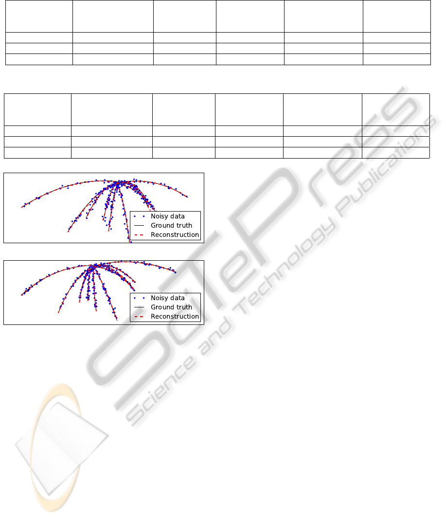
Table 2: Accuracy of the estimated parameters from noiseless data, compared with the ground truth. The errors are given in
terms of the average distance between the estimated parameters and the true parameters, the average error displays the mean
distance between the reconstructed trajectory and the ground truth.
Probability
of keeping a
measurement
Avg. measure-
ments per path
λ
λ
λ
0
error (cm) v
0
error, (m/s) radius error (mm) Avg. error (m)
0.5 653.16 1.11e-04 4.30e-06 3.45e-06 1.2e-06
0.1 131.08 2.54e-04 1.13e-05 9.85e-05 3.2e-06
0.05 66.15 1.09e-05 1.82e-06 8.81e-05 8.0e-07
Table 3: Like table 2, but with normal noise of σ = 5 added to the measurements.
Probability
of keeping a
measurement
Avg. measure-
ments per path
λ
λ
λ
0
error (cm) v
0
error, (m/s) radius error (mm) Avg. error (m)
0.5 651.73 4.19e+00 1.71e-01 2.35e-01 5.1e-02
0.1 129.43 8.93e+00 3.67e-01 4.22e-01 1.1e-01
0.05 66.98 1.08e+01 4.09e-01 5.52e-01 1.3e-01
Figure 1: Reprojection into the two virtual cameras of some
of the trajectories used in Table 3. The dotted line repre-
sents the noisy data, the solid line is the ground truth, and
the dashed line shows the trajectory reconstructed from the
noisy data.
and the mean distance between the reconstruction and
the ground truth trajectory. In Table 3, normal noise
with σ = 5 was added to the measurements. Figure
1 shows the reconstruction for some of the noisy tra-
jectories from 5% of the measurements. Even with so
few points, the reconstructed trajectory is remarkably
similar to the ground truth functions.
5.3 Trajectory Reconstruction and
Extrapolation
In (Zarrabeitia et al., 2012), a 2D quadratic poly-
nomial approximation was employed to track blood
droplets in the image plane. It was found that the
quadratic model was able to accurately predict the ex-
pected locations of the droplets within a very small
time window. It was also noticed that the quadratic
predictions broke down quickly after a few frames
without a measurement, or if too many measurements
were used to estimate the model.
Table 4 compares the accuracy of the reconstruc-
tion if only a small window of time is available. The
accuracy is measured as the average deviation from
the ground truth for the entire simulation time. This
allows us to evaluate the predictive capacity of each
simplified flight model, that is, how precisely each
model allows us to extrapolate from a small set of
measurements. We can see that the ODE models be-
haved significantly better than quadratic polynomial
model. The no drag model also behaved significantly
better than the quadratic polynomial model in the
noisy case for the first two columns. Figure 2 sug-
gests why this happens: having more degrees of free-
dom, the quadratic polynomial model may overfit the
noise in the data, resulting in a very inaccurate extrap-
olation. This is consistent with the prediction break-
down observed in (Zarrabeitia et al., 2012). Without
noise (Figure 3), both ODEs were able to accurately
reconstruct the entire trajectory using only the first
0.1s of flight. The polynomial models also behaved
much better with noiseless data, but they were still
significantly worse than the ODEs.
6 AN APPLICATION TO THE
BLOOD TRAJECTORY
RECONSTRUCTION PROBLEM
Our main reason for developing the nonlinear recon-
struction method (11) was the study of the motion pa-
rameters of blood droplets. Particularly, we wish to
DropletTrackingfromUnsynchronizedCameras
463
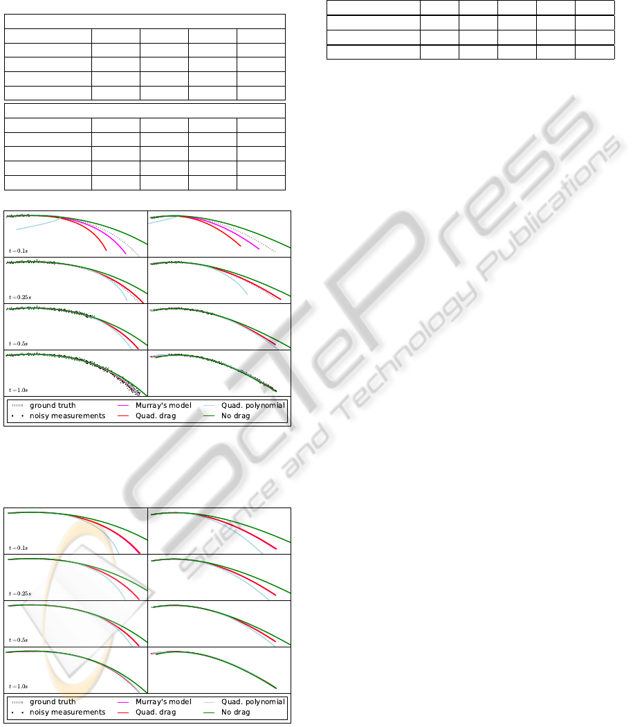
Table 4: Prediction accuracy, with noise (top) and without
noise (bottom). The values represent the mean distance, in
meters, between the ground truth and the estimated model
over the entire trajectory, when only measurements corre-
sponding to the first 0.1s, 0.25s,0.5s and 1.0s of flight are
used.
With noise
time (s) 0.1 0.25 0.5 1.0
Murray’s model 0.0041 0.00083 0.00022 9.9e-05
Quad. drag 0.005 0.00096 0.00024 9.9e-05
Quad. polynomial 0.12 0.0075 0.0011 0.00046
No drag 0.0048 0.0027 0.0032 0.0041
Without noise
time (s) 0.1 0.25 0.5 1.0
Murray’s model 1e-05 1e-05 1e-05 1e-05
Quad. drag 7.9e-05 5.6e-05 2.6e-05 1.3e-05
Quad. polynomial 0.00086 0.00071 0.0005 0.00032
No drag 0.0018 0.0019 0.0023 0.0029
Figure 2: Reconstruction of a trajectory from a small
amount of noisy data (σ = 5). Note how, in the first row,
the quadratic polynomial model overfits the available data,
causing it to behave extremely badly outside of the interval.
Figure 3: Like Figure 2, but without any noise added to the
data.
construct a framework to validate whether (12) is a
Table 5: Average deviation from the ground truth, in cm,
using different reconstructions from noisy data, with detec-
tion accuracy of 0.1, 0.25, 0.5, 0.75 and 1.0. 50 random
trajectories of 1s duration with normal noise (σ = 5) were
used.
Method \ Accuracy 0.1 0.25 0.5 0.75 1.0
Triangulation 33.87 34.78 34.39 34.58 34.22
3D optimization 61.63 11.02 3.192 2.154 1.324
Unsynchronized 5.165 2.961 2.015 1.504 1.285
good approximation, and whether simpler approxima-
tions are suitable under some constraints. An exper-
imental apparatus to measure blood droplet trajecto-
ries is described in (Zarrabeitia et al., 2012; Murray,
2012). Furthermore, (Murray, 2012) used these tra-
jectories to develop and validate (12). However, as
tables 3 and 4 show, the accuracy of the reconstruc-
tion from noisy data depends greatly on the number
of measurements available. It is thus essential to max-
imize the number of useful measurements.
The approach in (Zarrabeitia et al., 2012) is only
able to retrieve 3D coordinates for simultaneous mea-
surements. Due to the noise and random misdetec-
tions, even perfectly synchronized cameras cannot
guarantee finding a pairing for most of the trajectory.
Moreover, the sensitivity of the stereo reconstruction
with respect to the measurements in the image plane
increases with the distance of the target to the camera
center. Conversely, this means that there is a region
around each reconstructed point that produces very
similar measurements, and the size of this region in-
creases with the depth of the target. Fitting a model to
these reconstructions ignores that they are not equally
accurate.
Table 5 illustrates this issue. The synchronized
reconstruction (triangulation) solves the location of
each point independently, using equation (7). Observe
the very high average deviation from the ground truth.
The 3D optimization consists of fitting the model (12)
to the synchronized 3D reconstruction. It produces a
significant improvement over equation (7), though it
still depends heavily on the accuracy of the detector.
Finally, the unsynchronized reconstruction proposed
in this paper, using Murray’s model (12) produces a
significantly better approximation to the ground truth.
Ground truth is not available with real trajectories,
such as those measured by (Zarrabeitia et al., 2012)
(Figure 4). This makes it impossible to directly evalu-
ate the reconstruction accuracy. Instead, we can eval-
uate the prediction accuracy of the models. Figure 5
illustrates the reconstruction of a path from real mea-
surements obtained in (Zarrabeitia et al., 2012). The
droplet was recorded for about 0.5s, one of the longest
trajectories in that experiment. This makes it ideal for
evaluating the predictive power of the model, by fit-
ICPRAM2013-InternationalConferenceonPatternRecognitionApplicationsandMethods
464
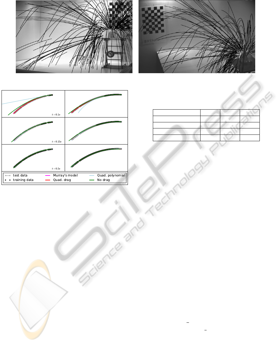
Figure 4: 2D trajectories measured by (Zarrabeitia et al., 2012).
Figure 5: Reconstruction of a real trajectory. Note that, con-
sidering only the first 0.1s of flight (top), the ODE models
were a near perfect fit for the overall trajectory, while the
quadratic polynomial model behaved badly. Also note that
because the noise is significantly lower than that of figure 2,
the reconstructions with t = 0.15 are nearly indistinguish-
able.
ting only a small window of time and comparing the
predictions with the actual measurements. The figure
shows that even with very few data points, the ODE
models were able to accurately predict the entire tra-
jectory.
A more complete test is summarized in Table 6.
This test was run over all the trajectories with at least
100 measurements per camera captured during a sin-
gle experiment. The errors shown are the average of
the distances, in pixels, between the predictions and
the measurements in the image plane. With incom-
plete data, the ODE models behaved significantly bet-
ter than the polynomials.
6.1 A Note about Outliers
When dealing with a real detector, such as the one
described in (Zarrabeitia et al., 2012), outliers are
likely to occur. In particular, the parabolic tracker
from (Zarrabeitia et al., 2012) tends to produce out-
Table 6: Prediction accuracy for real paths. Because ground
truth is not available, the errors are given in terms of pixels
in the image plane.
Model \ time (s) 0.1 0.15 0.5
Murray’s model 0.058 0.042 0.016
Quad. drag 0.12 0.048 0.013
Quad. polynomial 0.75 0.2 0.013
No drag 1.4 0.082 0.03
liers at the beginning of the trajectories, when there
is not enough data to find the quadratic coefficients.
Outliers may also appear near the end of the trajec-
tory, when the tracker, unable to find a new mea-
surement, may consume instead some blob near the
expected location. Most notably, the this also oc-
curs when the liquid droplet impacts a surface, as the
tracker may try to follow the bouncing particles be-
fore giving up (Figure 6, top left).
Both the linear approach (9) and the nonlinear (11)
are sensitive to outliers. In the linear case, they can be
handled with RANSAC, as we only need to solve a
small system of equations for each guess. However,
because our use of (9) is limited to computing a rough
initial guess for the Levenberg-Marquardt iteration,
we don’t need to filter out the outliers at this stage.
For the nonlinear case, RANSAC is prohibitively
expensive, as it would require to solve a nonlinear op-
timization problem with a differential equation as the
target function, for each candidate subset. Instead, we
follow a 2-pass approach (Figure 6): we use a robust
loss function, such as Huber loss, rewriting (11) as
ˆ
α
α
α = min
α
α
α
∑
hx
i
,P
i
,t
i
i∈M
H
δ
(x
i
− ϕ
i
(L
α
α
α
(t
i
))) (18)
H
δ
(x) =
1
2
x
2
if |x| < δ
δ(|x| −
δ
2
) otherwise.
(19)
to find the outliers (top), followed by another opti-
mization pass with square loss, considering only the
inliers and using the solution of (18) as the initial
guess (bottom).
DropletTrackingfromUnsynchronizedCameras
465
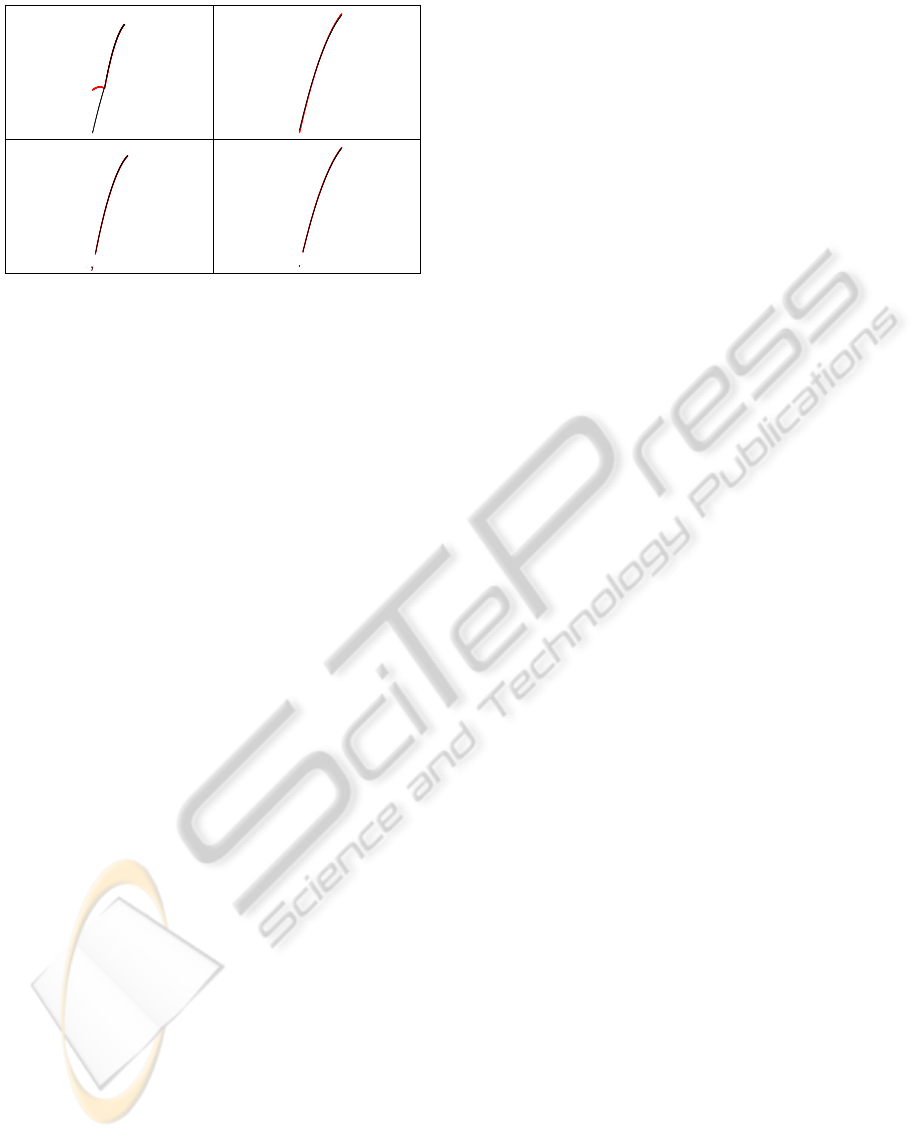
Figure 6: Outlier detection. A first pass fits the ODE pa-
rameters using a robustified loss function (top). The outliers
are then discarded and a second pass computes the final fit
(bottom). The original data is represented in red, the ODE
solution is overlaid in black.
7 CONCLUSIONS
We propose a method capable of estimating the 3D
path of a particle from a set of unsynchronized multi-
view image measurements. Our method is able to reli-
ably reconstruct the 3D trajectory of a particle—given
a parametrized model L
α
α
α
(t) describing its motion—
even in the presence of occlusions, misdetections and
misclassifications. Unlike other attempts that rely
upon motion models to improve 3D estimation accu-
racy, the proposed method makes no linearity assump-
tions about the motion model.
We applied the proposed method to the problem
of estimating the 3D trajectories of blood droplets
as they move through the air under the influence of
drag and gravity. Physical experiments that were car-
ried out to record these blood droplets are described
elsewhere (Zarrabeitia et al., 2012). We also gen-
erated synthetic dataset that faithfully mimics those
captured from the physical experimental setup men-
tioned above. The synthetic dataset allowed us to
evaluate the proposed approach under controlled set-
tings. We compared the four motion models described
in the previous section and we found that the polyno-
mial motion models fair poorly at the task of extrapo-
lation, i.e., estimating the full 3D trajectory of a par-
ticle given a small set of initial measurements. ODE
based motion models, on the other hand, correctly ex-
trapolated the 3D trajectory of a particle even in the
presence of noisy measurements. We achieved simi-
lar results for the real dataset.
Our results summarized in Table 5 are both ex-
citing and encouraging. We conclude that 3D recon-
struction via triangulation (using synchronized mea-
surements) often exaggerates measurement errors, af-
fecting 3D trajectory estimation. The proposed tech-
nique side-steps this issue by solving for both the 3D
trajectory of a particle and its motion model concomi-
tantly. We show that the proposed method outper-
forms the traditional triangulation based 3D trajectory
reconstruction approach.
REFERENCES
Aggarwal, S. and Peng, F. (1995). A review of droplet
dynamics and vaporization modeling for engineering
calculations. Journal of engineering for gas turbines
and power, 117(3):453–461.
Hartley, R. and Zisserman, A. (2004). Multiple view geom-
etry in computer vision. Cambridge University Press,
2
nd
edition.
Liu, A. B., Mather, D., and Reitz, R. D. (1993). Modeling
the effects of drop drag and breakup on fuel sprays.
NASA STI/Recon Technical Report N, 93:29388.
Murray, R. (2012). Computational and laboratory investi-
gations of a model of blood droplet flight for forensic
analysis. Master’s thesis, University of Ontario Insti-
tute of Technology.
Park, H., Shiratori, T., Matthews, I., and Sheikh, Y. (2010).
3d reconstruction of a moving point from a series of
2d projections. Computer Vision–ECCV 2010, pages
158–171.
Peng, F. and Aggarwal, S. K. (1996). Droplet motion un-
der the influence of flow, nonuniformity and relative
acceleration. Atomization and Sprays, Vol. 6:42–65.
Raymond, M. A., Smith, E. R., and Liesegang, J. (1996).
The physical properties of blood—forensic consider-
ations. Science & Justice: journal of the Forensic Sci-
ence Society, 36(3):153–160.
Zarrabeitia, L. A., Aruliah, D. A., and Qureshi, F. Z.
(2012). Extraction of blood droplet flight trajectories
from videos for forensic analysis. In ICPRAM 2012
- Proceedings of the 1st International Conference on
Pattern Recognition Applications and Methods, vol-
ume 2, pages 142–153. SciTePress.
ICPRAM2013-InternationalConferenceonPatternRecognitionApplicationsandMethods
466
