
A Geometrical Refinement of Shape Calculus Enabling Direct Simulation
Federico Buti, Flavio Corradini, Emanuela Merelli and Luca Tesei
School of Science and Technology, University of Camerino, Via Madonna delle Carceri 9, Camerino, Italy
Keywords:
Process Calculi, Spatial Simulation, Calculus Refinement, Computational Biology.
Abstract:
The Shape Calculus is a bio-inspired timed and spatial calculus for describing 3D geometrical shapes moving
in a space. Its purpose is twofold: i) modelling and formally verifying (not only) biological systems, and ii)
simulating the models for validation and hypothesis testing. The original geometric primitives of the calculus
are highly abstract: the associated simulator needs to attach a lot of code to the model specification in order
to perform an effective simulation. In this work we propose a calculus refinement in which a detailed 3D
characterization of the geometric primitives is injected into the syntax of the calculus. In this way, models
written with the new syntax can be directly simulated.
1 INTRODUCTION
Systems Biology (Kitano, 2002) could affect quite
deeply our everyday life in the next few years. Mod-
elling and computer simulation are rapidly changing
the way in which biological phenomena and processes
are studied. Contrasted to in vivo and in vitro experi-
mentations, in silico (i.e. simulation) experimentation
is cheaper, faster and much less expensive.
In silico experimentation is increasingly used,
from the prediction of pathological phenomena
(Grupe et al., 2001) to the tailoring of medical treat-
ments based on the characteristics of an individual
patient (Manos et al., 2008; Taylor et al., 1999) to
the application of nanotechnologies for the diagnosis,
prevention and treatment purely from a preventative
state (Lim, 2004; Kumar, 2007; Torchilin, 2006). The
final aim is to identify and stop potential sources of
disease/illness, such as cancer, before they even get
started (Ferrari, 2005; Kawasaki and Player, 2005).
In the context of this important challenge raised
by Systems Biology, computer scientists have started
to contribute by adapting (computational) models and
languages, originally thought for the design and the
analysis of hardware/software systems, to biologi-
cal systems. This adaptation process has revealed
that some of the languages, although general-purpose,
needed to be expanded with concepts and characteris-
tics typical of biological modelling. One of these fea-
tures is surely space, considered both in a topological
and a geometrical way. It is indeed well-known that
space and physical concepts like space occupancy,
space subdivision, crowding and co-localization play
a fundamental role in determining bio-interactions,
for instance at the cellular level (Takahashi et al.,
2005). Crowding, in particular, may lead to signifi-
cant alterations of biochemical or biological recogni-
tion processes at the molecular level (Minton, 1998)
and affects folding and refolding of proteins, i.e. the
process by which a protein structure assumes its func-
tional shape or conformation (van den Berg et al.,
1999).
Despite this, most of the modelling and the sim-
ulation approaches available today tend to assume a
homogeneous distribution of entities in space and to
abstract away specific spatial information. The Shape
Calculus (SC) (Bartocci et al., 2010a; Bartocci et al.,
2010b) has been proposed as a process calculus with a
rich set of primitives to describe mainly, but not only,
biological phenomena. The main characteristics of
this calculus are that it is spatial — with a 3D ge-
ometric notion of space — and it is shape-based, i.e.
entities have geometric simple or complex shapes that
affect the possible interactions with other entities.
Formal SC models, i.e. process specifications, are
currently used as a stub code for the associated sim-
ulation environment BIOSHAPE (Buti et al., 2010a;
Buti et al., 2011b). However, the original SC 3D char-
acterization of shapes and spatial channels is highly
abstract and its bond with the actual geometrical data
structures and code libraries used in BIOSHAPE is
quite loose.
In this work we provide a different, more detailed
and simulation-oriented syntax of the calculus. The
218
Buti F., Corradini F., Merelli E. and Tesei L..
A Geometrical Refinement of Shape Calculus Enabling Direct Simulation.
DOI: 10.5220/0004060802180227
In Proceedings of the 2nd International Conference on Simulation and Modeling Methodologies, Technologies and Applications (SIMULTECH-2012),
pages 218-227
ISBN: 978-989-8565-20-4
Copyright
c
2012 SCITEPRESS (Science and Technology Publications, Lda.)

Table 1: A comparative table containing the Shape Calculus original syntax (left) with highlighted abstract geometric primi-
tives and the new, simulation-oriented, syntax (right).
Basic Shapes σ =
H , m, p, v
σ = hW, m, v, ω, s, T i
Shapes S ::= σ
S h X i S S ::= σ
S h{ϕ
1
, ϕ
2
}iS
Behaviours
B ::= nil
hα, X i.B
ω(a, X ).B
ρ( L
∗
).B
ε(t).B
B + B
K
B ::= nil
hα, {ϕ
1
, . . . , ϕ
n
}i.B
ω(a, {ϕ
1
, . . . , ϕ
n
}).B
ρ(L
∗∗
).B
ε(t).B
B + B
K
3D Processes P ::= S[B]
Pha, X i P P ::= S[B]
Pha, {ϕ
1
, ϕ
2
}iP
3D Networks N ::= Nil
P
N kN N ::= Nil
P
N kN
∗
where L = {ha, X i | ha, X i is a channel}
∗∗
where L = {ha, {ϕ
1
, . . . , ϕ
n
}i | ha, {ϕ
1
, . . . , ϕ
n
}i is a channel}
final aim is to produce a refinement of the language
that syntactically incorporates a finitary, complete de-
scription of the geometry involved. This will make
the bond between the specification language and the
simulating code more tight, thus allowing the direct
simulation of the models. It is worth noting that the
resulting refined language does not loose the neces-
sary abstraction needed to perform formal verifica-
tion. In Table 1 we show, on left, the original grammar
of SC where the abstract geometrical representations
are highlighted. Throughout the paper we briefly ex-
plain and then revisit all the syntax categories and for
each of them we introduce a finitary geometrical rep-
resentation, summarized on the right.
The rest of the paper is structured as follows: Sec-
tion 2 summarizes some basic concepts about the cal-
culus, highlighting its limitations w.r.t. a computa-
tional simulation setting, Section 3 briefly introduces
the simulation tool BIOSHAPE, Section 4 defines the
new 3D representation of shapes, Section 5 describes
the new syntax to define the behaviours associated to
shapes, Section 6 provides some insight about the im-
plementation of the new syntax in the simulation envi-
ronment. Finally, Section 7 traces ongoing and future
work.
2 THE SHAPE CALCULUS
The general idea of the SC is to consider a 3D space in
which shapes move and interact. Shapes can be sim-
ple 3D generic geometric primitives (cubes, cylinders,
etc.) or complex (even non convex) compositions of
simpler shapes. While time flows, shapes move ac-
cording to their velocity vectors that can change over
time due to a general motion law (e.g. for an electro-
magnetic field), Brownian motion or collisions occur-
ring between shapes.
Let us now briefly and informally summarize the
semantics of the language passing through all the syn-
tax categories (always refer to Table 1); the full for-
mal semantics can be found in (Bartocci et al., 2010a;
Bartocci et al., 2010b). Basic shapes are represented
as tuples containing a set H of 3D points defining the
shape (with a non-specified finitary representation), a
mass m ∈ R
+
, a point p in 3D representing the centre
of mass and a velocity v. Composed shapes (Sh X iS)
are generated by glueing together basic or composed
shapes on touching common surfaces ( h X i, again
with a non-specified finitary representation).
A shape (S) together with a behaviour (B) defines
a 3D process (S[B]), the basic building block of a SC
model. 3D processes can also be composed processes
(Pha, X i P) that are such that their original shapes are
glued together on a certain bound (ha, X i ) and their
original behaviours operate in parallel (in Figure 1 we
show an example of two 3D processes interacting).
Action prefixing in behaviours (hα, X i.B) represents
an open channel (hα, X i) associated to a shape.
Channels are derived from classical CCS (Milner,
1982) channels, where α is the channel name, in-
tended as a type for binding certain species, and X
is a certain region on the surface of the associated 3D
shape in which the channel is “active”. Channels de-
termine how a process responds to a collision. One
of the first motivations of the calculus comes from the
dynamics of molecules inside a cell, thus behaviours
mimic what it is known to happen in biochemical re-
actions
1
. Like molecules, which can bind on a partic-
ular portion of their physical shape, 3D processes can
bind if they collide on compatible surfaces.
A collision happening on compatible channels,
i.e. having a corresponding CCS name/co-name and
such that the intersection between their active surfaces
is not empty, results in an inelastic response; the col-
liding processes bind and become a compound new
process moving in a different way and having a differ-
ent behaviour. Collisions on non-compatible channels
1
However the calculus has then been demonstrated to
be general enough to be applied to a lot of scenarios, at
different scales, in different fields.
AGeometricalRefinementofShapeCalculusEnablingDirectSimulation
219

Figure 1: Two 3D processes get near after an interval t (left) and then clash on compatible surfaces X and Y . Hence, an
inelastic collision occurs and a binding is generated on surface Z = X ∩Y (centre). After some other time, the compound
shape weakly split and the components move away (right).
result in an elastic response, i.e. they bounce away.
Compound processes can split weakly (ω(a, X ).B)
by non-deterministically releasing a previously estab-
lished bond, or “react” (operator ρ( L ).B), by split-
ting in as many pieces as the products of the reaction
are (i.e. the bonds in L ). Non-determinism in be-
haviours (B + B) permits the opening of several chan-
nels and the enabling of different splitting behaviours
at the same time. The timed operator ε(t).B waits t
time units before proceeding with the continuation B.
Finally, the process variable K is needed to specify
recursive behaviours. A complete SC model corre-
sponds to a 3D Network, i.e. the parallel composition
of several 3D processes that are intended to evolve in
the same space.
Figure 2: A continuous trajectory (blue) approximated via
a polygonal chain (orange).
Time evolves discretely by timesteps of duration
∆, also called movement time step. At the beginning
of each timestep the velocity of the shapes is updated
by means of a so called steer function and remains
constant until the subsequent timestep update. Both
velocity update and evolution of shapes are repre-
sented as an update of the shape tuple(s). The result-
ing polygonal chain describing the movement of the
shape approximates a corresponding continuous tra-
jectory of the shape (see Figure 2). This approach is
computationally cheaper than modelling continuous
trajectories (Ericson, 2005) and quite faithful for rea-
sonably small ∆. If a collision occurs, the timestep
is shortened to the instant before the shapes start to
interpenetrate (so called first time of contact or Ftoc)
and the collision is resolved, according to what stated
above for elastic and inelastic collisions. After the
resolution a new timestep begins. The calculus does
not embed a specific algorithm for Ftoc calculation
and resolution so that any desirable collision detec-
tion/collision resolution system can be adopted.
3 BIOSHAPE: SHAPE CALCULUS
MODELS AT WORK
BIOSHAPE (Buti et al., 2010a; Buti et al., 2010b;
Buti et al., 2011a; Buti et al., 2011b) is a modelling
and simulation environment that has been engineered
in the perspective of being uniform, particle-based,
3D space- and 3D geometry-oriented. A shape in
BIOSHAPE, being the concept inherited from the SC,
can be either a basic one (a convex closed polyhedron)
or a correctly composed one (a generic polyhedron).
Note that differently from SC, here only the specific
class of polyhedra is used for shapes. The basic ele-
ment of a simulation is the entity, corresponding to a
SC 3D process. In other terms, an entity owns a par-
ticular 3D shape and a specific behaviour along with
an associated physical motion law (the latter repre-
sented by an instance of the so called Driver class).
The behaviour of every entity, i.e. the way in which it
interacts with other entities and with the environment,
is defined partially through the SC behaviour, and par-
tially through Java programming. Hence, the SC acts
as a sort of stub code for the simulation, but there is
not a tight bond between the specification language
and the implementation.
In the SC, shapes are defined w.r.t. a global 3D
coordinate system that we call world space, whereas
binding sites are always defined w.r.t. a system local
to the shape. This approach poses a performance is-
sue: the same redundant geometry structure is main-
tained for each instance of a 3D process whereas it
would be sufficient to manage the position and the
orientation of each process referring to a unique in-
SIMULTECH2012-2ndInternationalConferenceonSimulationandModelingMethodologies,Technologiesand
Applications
220

stance of the geometry structure. The simulator solves
this problem by following a classical approach of
rigid body simulations (Baraff, 1997). The shapes
are defined in terms of a fixed and unchanging space
called body space. A suitable affine transformation
must be applied to move (i.e. translate and rotate) the
shape points from the body-space description into the
world space description. An affine transformation T
is any transformation that preserves collinearity (i.e.
all points lying on a line initially still lie on a line
after transformation) and ratios of distances (e.g. the
midpoint of a line segment remains the midpoint after
transformation) and can be used to describe both ro-
tations and translations, along with other transforma-
tions. Affine transformations are finitely represented
by a 4x4 matrix. Thus, using this approach, the ge-
ometry is defined only once and acts as a sort of tem-
plate which is then instanced to real shapes by defin-
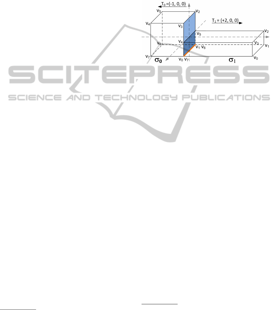
ing different affine transformations. Figure 3 shows a
shape template that is defined at the origin and then
two shape instances, σ
0
and σ
1
, with different po-
sitions and orientations, generated applying suitable
transformations T
0
and T
1
. Obviously, both instances
will refer to the same, unique, shape template.
Figure 3: The declaration of a shape template (left) and its
instantiation into two shapes (right), σ
0
and σ
1
with differ-
ent positions and orientations due to their transformations
T
0
and T
1
.
Note that the description of the shape in body
space is required to be such that the centre of mass of
the body lies at the origin. Despite not being a strict
requirement, this choice simplifies operations over the
shapes and their transformations.
Whereas in the SC no specific collision detection
algorithm is defined, in BIOSHAPE a two-phase al-
gorithm based on V-Clip algorithm (Mirtich, 1998) is
adopted in order to establish whether shapes collide
and when (Ftoc).
To handle the computational cost of simulating 3D
shapes moving in an environment, BIOSHAPE has
been engineered to support both the cluster and the
distributed computational approaches. BIOSHAPE
is based on the agent-based Java framework Her-
mes
2
, a middleware supporting distributed applica-
2
HermesV2 official site: http://hermes.cs.unicam.it
tions and mobile computing — see (Corradini and
Merelli, 2005) for further information. Such frame-
work enables BIOSHAPE to split the simulated space
into portions which are assigned to different commu-
nicating computational nodes.
For other features of the modelling and simulation
environment BIOSHAPE see (Buti et al., 2010a; Buti
et al., 2010b; Buti et al., 2011a; Buti et al., 2011b).
4 NEW SHAPES
The usage of the calculus in a simulation setting re-
quires that the boundary of a shape is correctly de-
scribed and binding sites are unambiguously identi-
fied. However, as explained in the introduction, the
calculus poses some limitations to its direct usage in a
simulation setting: the geometrical representation of
a shape is, in fact, unspecified and the identification
of common touching surfaces is vague. These limits
call for a different, more detailed, representation of
the shapes in which all the geometric elements com-
posing them can be finitely embedded into the syntax
and unequivocally identified.
Since interactions occur on compatible shape sur-
faces, we are interested in characterizing a shape in
terms of its boundary more than in terms of all its
constituent points, as done in the original syntax. To
this purpose, as a first step, we discard the generic
primitives mentioned in Section 2, to focus solely on
polyhedral shapes.
Polyhedra (or polyhedrons) are one of the most
widely used geometric solids in computer-modelling
applications (Ericson, 2005). In particular, they are
used to model real-world objects in computer graph-
ics and obstacles in robotic systems. Given a poly-
hedron W in 3D, it is a set of points whose boundary
consists of planar pieces called facets (faces in 3D).
The faces of W meet along straight line segments,
called edges while its edges meet at vertices. Faces,
edges and vertices of a polyhedron are called its fea-
tures — see (Hoffmann, 1989; M
¨
antyl
¨
a, 1988) for a
deeper introduction on polyhedra. We are particularly
interested in polyhedra which are convex and closed
because these will be the new basic shapes.
4.1 Basic Shapes
A convex polyhedron is a solid for which the entire
figure lies on one side of the plane of each constituent
polygon. Equivalently, we can say that a polyhedron
is convex iff it contains the entire segment between
any pair of its points. Since a convex polyhedron lies
on one side of the plane of each of its faces, it is easy
AGeometricalRefinementofShapeCalculusEnablingDirectSimulation
221
(a) (b)
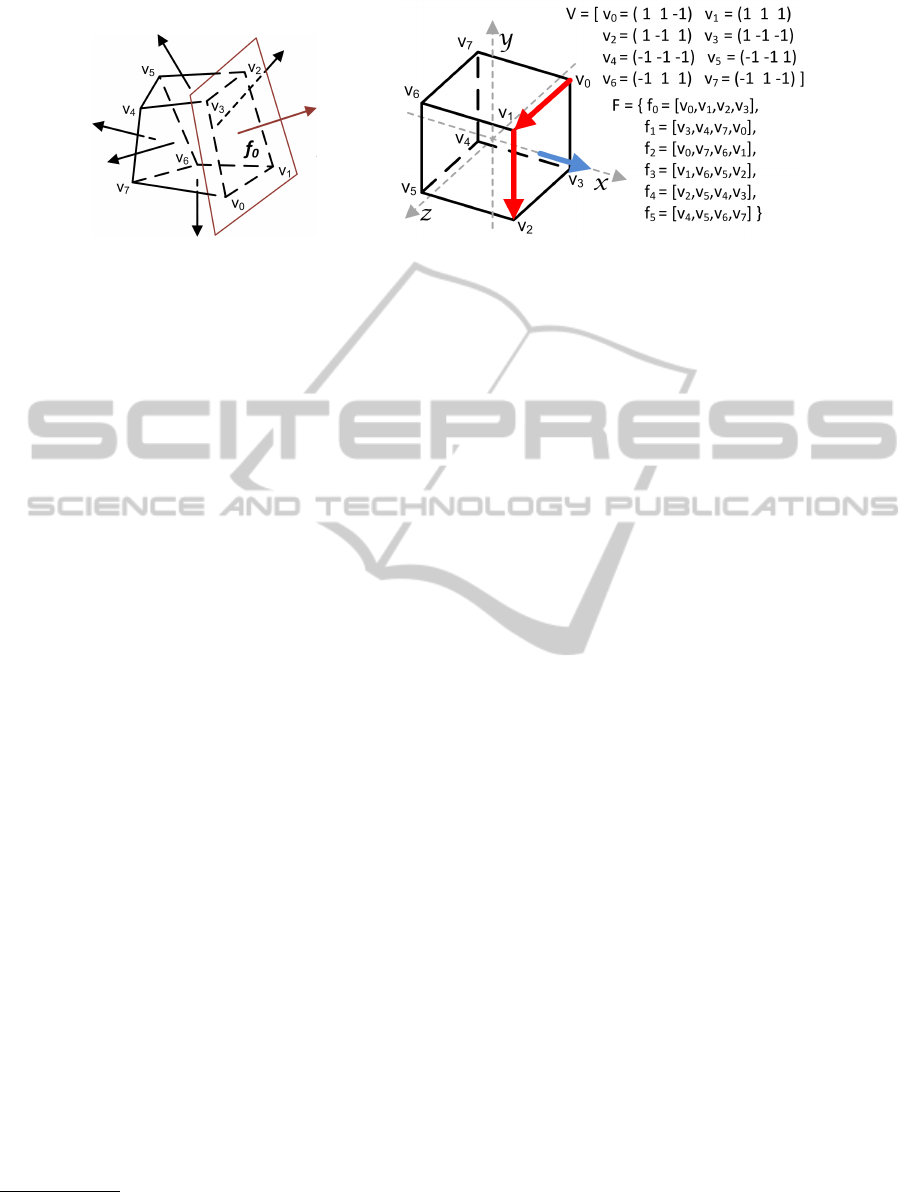
Figure 4: A convex polyhedron (a) with the faces outward normals. A cube description (b) in terms of an IFS; note the
example normal (blue) automatically calculated by cross product of the first two edges (red) of the corresponding face.
to show that at most two faces meet at any edge and
that any interior point of one face cannot belong to
another face. A convex polyhedron is closed if all its
edges belong to exactly two faces.
In a convex polyhedron the planes of all its faces
are support planes. A support plane is a plane hav-
ing at least one point in common with the figure and
such that the entire figure lies in one of the two half-
spaces bounded by the plane
3
. In particular, the di-
rection of a support plane is always the direction of
its outward normal. Thus, the direction of a face of a
polyhedron is the direction of the same outward nor-
mal vector, i.e. the direction pointing away from the
face. In Figure 4(a) a convex polyhedron is shown,
along with the support plane for the face [v
0
, v
1
, v
2
, v
3
]
and the outward normal; normals for other faces are
also represented. Looking at the picture, we can intu-
itively identify an important property captured by the
following theorem — see (Aleksandrov, 2005) for the
proof:
Theorem 1 (Polyhedron and Support Planes). Every
convex closed polyhedron is determined by the planes
of its faces and their outward normals.
Hence, we can correctly define a convex, closed
polyhedron in terms of its faces, which in turn can
be defined in terms of the composing vertices and the
normal.
For the purpose of this paper, we adopt the ap-
proach of indexed face set (IFS), a general data struc-
ture often used in computer graphics (Hartman and
Wernecke, 1996; Murray and VanRyper, 1996). How-
ever, since we want to use names in the syntax, we
slightly adapt this approach as described below.
In an IFS representation, a sequence of points is
followed by the definition of a sequence of faces.
Each face is a list of indices referring to the se-
3
Following the definition, it is possible to define support
planes also for vertices and edges. However they are of no
interest in this work.
quence of vertices. The latter are stored in a counter-
clockwise (ccw) order by default, making explicit
declaration of normals unnecessary. Indeed, the vec-
tor normal is automatically calculated via the cross
product of two vectors connecting the first vertex of
the face to the second, and the second to the third.
Edges must be derived implicitly from adjacent ver-
tices in the enumeration of the vertices of a face. Pic-
ture 4(b) shows an example of IFS for a cube of side
two. The cube is generated with its centre at the origin
(as suggest in Section 3) so that its vertices are posi-
tioned at a maximal distance of one in all of the three
coordinates. Note also the normal calculated as de-
scribed above (i.e. (v
3
−v
2
)× (v
0
−v
3
)). A clockwise
order of the vertices would have generated negated
vectors and thus a negated normal, i.e. with opposite
direction, and the resulting polyhedron would have
not been closed.
Let us formalize all these concepts into the SC set-
ting. We are interested in correctly identifying all the
features of a polyhedron. Hence, we enrich the nota-
tion of the IFS by adding a name to each vertex and
by defining faces as tuples over these names.
Let P = R
3
be the sets of positions. Let NamesV
be an infinite numerable set of names {u, v, w, . . . } that
will be used to denote positions. Vertices denotes the
set of all tuples of length one composed by names
in NamesV. These tuples will be used to represent
vertex features. For instance, face f
0
in Figure 4(a)
has the following four vertices: [v
0
], [v
1
], [v
2
] and [v
3
].
We will range over both elements of NamesV and
Vertices by u, v, w, . . . since the denoted element can
be always understood by the context. Edges, ranged
over by e, e
0
, e
1
, . . . denotes the set of all tuples of
names in NamesV with length two. These will rep-
resent the edge features. For instance, face f
0
in Fig-
ure 4 has the following four edges: [v
0
, v
1
], [v
1
, v
2
],
[v
2
, v
3
] and [v
3
, v
4
]. Faces, ranged over by f , f
0
, f
1
, . . .
denotes the set of all tuples of names in NamesV, with
SIMULTECH2012-2ndInternationalConferenceonSimulationandModelingMethodologies,Technologiesand
Applications
222

length greater than or equal to three
4
, representing
face features of our shapes. For instance, face f
0
of
Figure 4(a) can be represented by [v
0
, v
1
, v
2
, v
3
].
Note that, each type of feature can be charac-
terised by its dimension, which can be defined infor-
mally as the minimum number of coordinates needed
to specify any point within it. Hence, vertices have
dimension zero, edges have dimension one and faces
have dimension two.
Note also that, as we explained above, the order
of the names in the tuples matter. However, since a
face is basically a sequence of its vertices (listed in
the tuple), there are multiple tuples denoting the same
face, one for each composing vertex. This naturally
leads to the definition of an equivalence relation in
Faces.
Definition 1 (Rotation Equivalence). Given a face
representation as a tuple f = [v
1
, . . . , v
n
], then the tu-
ple f
0
= [v
n
, v
1
, . . . , v
n−1
] is an equivalent representa-
tion of f . We will write f ≡ f
0
.
For instance, the face of the polyhedron
of Figure 4(a) can be equivalently represented
by [v
0
, v
1
, v
2
, v
3
], [v
3
, v
0
, v
1
, v
2
], [v
2
, v
3
, v
0
, v
1
] and
[v
1
, v
2
, v
3
, v
0
].
Finally, we define the set Features of all features,
ranged over by ϕ, ϕ
0
, ϕ
1
, . . . as the union Vertices ∪
Edges ∪Faces. Now we need to introduce some func-
tions that will be useful in the following.
Definition 2 (Downgrade and Closure Functions).
Given e ∈ Edges, f ∈ Faces and given V ⊂
Vertices, E ⊂ Edges and F ⊂ Faces, we define down-
grade functions dg(e) , {[v] | e = [v
1
, v
2
] ∧ v ∈
{v
1
, v
2
}} and dg( f ) , {[v
i
, v
j
] | f = [v
0
, . . . , v
n−1
] ∧
i ∈ {0, . . . , n − 1} ∧ j = i + 1 mod n}. We also lift
the functions dg on sets: dg(E) ,
S
e∈E
dg(e) and
dg(F) ,
S
f ∈F
dg( f ). Finally, we define a closure op-
erator on a set of Features Φ:
closure(Φ) ,
{v | v ∈ Φ ∧ v ∈ Vertices} ∪
{e | e ∈ Φ ∧ e ∈ Edges} ∪
{ f | f ∈ Φ ∧ f ∈ Faces} ∪
dg({e | e ∈ Φ ∧ e ∈ Edges}) ∪
dg({ f | f ∈ Φ ∧ f ∈ Faces}) ∪
S
e∈dg({ f | f ∈Φ∧ f ∈Faces})
dg(e)
Downgrade functions are used to obtain a set of
features of lower dimension from features of higher
one. For instance, the application of the downgrade
function to face f
0
= [v
0
, v
1
, v
2
, v
3
] of polyhe-
dron of Figure4(a) returns the composing edges:
dg( f
0
) = {[v
0
, v
1
], [v
1
, v
2
], [v
2
, v
3
], [v
3
, v
0
]}. The same
applies to the edges, e.g. for e
0
= [v
0
, v
1
] in f
0
we have
4
Indeed, a face must be at least a triangle.
that dg(e
0
) = {[v
0
], [v
1
]}. The closure operator is used
to add to any given set of features all missing features
of lower dimensions that compose them. For instance,
consider the set Φ = { f
0
, [v
1
]}, then closure(Φ) =
{ f
0
, [v
0
, v
1
], [v
1
, v
2
], [v
2
, v
3
], [v
3
, v
0
], [v
0
], [v
1
], [v
2
], [v
3
]}.
We are now ready to introduce formally a convex
polyhedron described as an IFS.
Definition 3 (Convex Closed Polyhedron). Let V ⊂
Vertices be a finite set of vertices and let F ⊂ Faces
be a finite set of faces. The set W = V ∪F represents a
convex closed polyhedron iff all of the following con-
ditions hold:
1. |V | ≥ 4 and |F| ≥ 4
5
;
2. each tuple f ∈ F is composed only of vertices in
V ;
3. V is not a collinear set, i.e. the positions of the
vertices do not lie on a single line;
4. ∀ f ∈ F, f is a convex polygon;
5. ∀ f
i
, f
j
∈ F, it holds that f
i
6≡ f
j
, according to Def-
inition 1;
6. angles between any two edges in dg(F) are con-
vex, i.e. less than 180 degrees;
7. the Euler characteristic, i.e. χ = |V | − |dg(F)| +
|F| must be equal to 2.
The first condition is necessary, since the simplest
polyhedron which can be defined is a tetrahedron,
having exactly four vertices and four triangular faces.
Second condition ensures that the generated IFS con-
tains only faces whose vertices are available in the set
itself. Conditions 3-7 are sanity checks, needed to
guarantee that a generated IFS correctly describes a
convex closed polyhedron — see again (Aleksandrov,
2005) for deeper geometrical details.
Apart from tetrahedrons, other basic figures can
be defined according to the definition above, such
as cubes, parallelepipeds and generic convex prisma-
toids, i.e. prisms, antiprisms, pyramids, cupolas, frus-
tums and wedges. Other primitives, i.e. cones, cylin-
ders and spheres cannot be used directly but can be
approximated to corresponding polyhedral represen-
tations.
We are now ready to introduce the new basic
shapes of our calculus, following the previous defi-
nitions. Similarly to the approach described in Sec-
tion 3, we will use a convex closed polyhedron, as
defined in Definition 3, as a template, i.e. only one
data structure for one kind of W is created. Then, any
instance of the template can be obtained by applying
an affine transformation that will move the shape into
the world space. Moreover, we add a name for ba-
sic shapes that will create a namespace to give unique
5
By | · | we denote the cardinality of a set.
AGeometricalRefinementofShapeCalculusEnablingDirectSimulation
223
names to the feature of each instance. For example,
if in the template W there is a face f
0
= [v
1
, v
2
, v
3
, v
4
],
then in an instance s
0
the corresponding face will be
denoted by s
0
. f
0
= [s
0
.v
1
, s
0
.v
2
, s
0
.v
3
, s
0
.v
4
], where s
0
is the name of the instance.
Definition 4 (New Basic Shapes). A basic shape σ is
a tuple hW, m, v, ω, s, T i where W = V ∪ F is an IFS
representing a convex closed polyhedron as described
in Definition 3, m ∈
+
is the mass
6
, v is the translation
velocity, ω is the angular velocity, s is the name of
the basic shape taken from an infinite numerable set
of names NamesB and T is a transformation matrix
that moves the template W from the body space to the
world space of the model. We denote by T (W) the IFS
moved to the world space. All possible basic shapes
are ranged over by σ, σ
0
, σ
1
. . ..
Differently from the original definitions, now
shapes have also an associated angular velocity, i.e.
they can also rotate in addition to translate. While
time flows the position of each shape will be updated
by changing its affine transformation according to the
associated translation and rotation velocities.
Consider a cube whose geometry W
0
= V ∪ F
where V and F are the ones provided in Figure 4(b).
A correctly instanced cube σ is a tuple such as
the following: σ = hW
0
, m = 3, v = (2, 1, 1), ω =
(0, 0, 0), s
0
, T i where T is such that the shape does not
rotate and translate of a vector (2, 3, 1). The current
position of the cube can be derived by its transforma-
tion T and its position in the body space. Since the
geometry is defined in a body space with the centre
of mass in the origin, (2, 3, 1) corresponds also to the
current position of σ. Moreover, since the instance
has no angular velocity, it is only going to translate
by the amount specified by v.
4.2 Compound Shapes
Basic shapes can be glued together to form more com-
plex shapes, also non-convex ones. Intuitively, two
shapes can be attached if they do not interpenetrate
and at least one of their features touch in the world
space. Note that more than one feature from both
shapes may be touching, e.g. when two shapes are in-
volved in a perfect face-face collision such that also
edges and vertices are in contact. However, just one
feature of each shape may be involved, e.g. when the
shapes collide in a face-vertex case.
It is sufficient for our purposes to syntactically
specify just one feature from each of the composing
shapes, but with the requirement that it is with the
highest possible dimension.
6
We will always consider solid bodies with uniform
mass density.
Definition 5 (New 3D Shapes). The set of the new
3D shapes, ranged over by S, S
0
, S
1
. . ., is generated
by the grammar: S ::= σ
S h{ϕ
1
, ϕ
2
}iS where σ is a
new basic shape and ϕ
1
, ϕ
2
are two features, one from
each of the two glued shapes, such that they touch
without interpenetrating and they are of the highest
possible dimension.
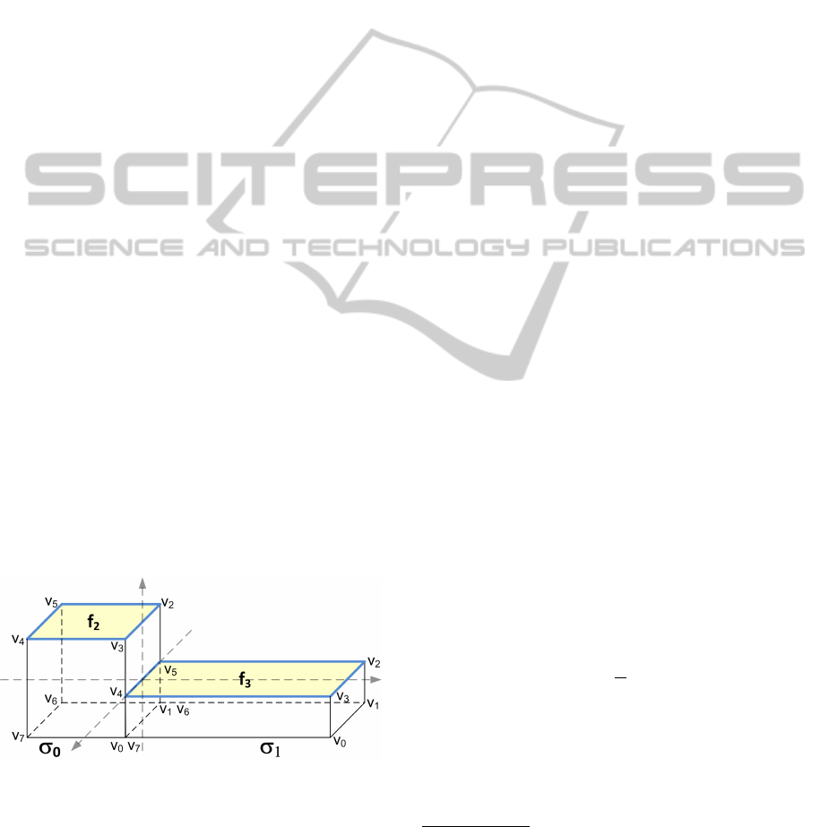
Figure 5: A compound shape S
0
, obtained by glueing to-
gether two basic shapes, σ
0
and σ
1
.
For example, with this definition, we can generate
a concave compound shape, as the one represented
in Figure 5. This shape is formed by an instance of
the cube template of Figure 4(b) and an instance of
a parallelepiped template W
1
. For the sake of brevity
we do not present the IFS defining the parallelepiped
but we assume that, like the cube, it has been defined
with the centre of mass in the origin and also that it
has sides of size 4, 1, 2, i.e. it is double the length of
the cube, half its height and has the same depth.
The final compound shape of Figure 5 is ob-
tained by generating the two instances and by
moving them on the x-axis according to the vec-
tors depicted in figure. The two instances are
represented by tuples: σ
0
= hW
0
, m
0
= 3, v
0
=
(2, 1, 0), ω
0
= (0, 0, 0), s
0
, T
0
i and σ
1
= hW
1
, m
1
=
3, v
1
= (2, 1, 1), ω
1
= (0, 0, 0), s
1
, T
1
i
7
. The glue-
ing features is the set of two faces touching at the
origin, (blue features in Figure 5) even if the two
shapes touch only on a portion of such features
(dark blue section in Figure 5). The features are
called s
0
. f
0
= [s
0
.v
0
, s
0
.v
1
, s
0
.v
2
, s
0
.v
3
, ] and s
1
. f
1
=
[s
1
.v
4
, s
1
.v
5
, s
1
.v
6
, s
1
.v
7
, ]. Hence, the final shape is
defined as S
0
= σ
0
h{s
0
. f
0
, s
1
. f
1
}iσ
1
. Note that, in
this case, it is not possible to select another set of
features. For instance, if we select edges s
0
.e
0
=
[s
0
.v
0
, s
0
.v
1
] and s
1
.e
1
= [s
1
.v
6
, s
1
.v
7
] (coloured or-
ange in the picture) we would not satisfy the require-
ment of the highest dimension.
7
The velocity vectors of the two shapes are the same,
this ensure that while moving they would not eventually in-
terpenetrate or move apart.
SIMULTECH2012-2ndInternationalConferenceonSimulationandModelingMethodologies,Technologiesand
Applications
224
5 NEW CHANNELS AND 3D
PROCESSES
Channels in SC represent active sites on the surfaces
of shapes on which a possible collision-driven inter-
action can occur. In the original syntax they are of the
form hα, X i where α is the channel name and X is a
surface of contact that must belong to the surface of
the shape in which the channel is opened. The name
α belongs to NamesC, ranged over by α, β, . . ., de-
fined as Λ ∪
¯
Λ where Λ is an infinite numerable set of
names a, b, c, . . . and
¯
Λ = { ¯a | a ∈ Λ}. The set X must
be substituted by a finitary representation. The nat-
ural candidate is a finite set of features belonging to
the shape in which the channel is embedded. To avoid
writing a long list of features one can use the closure
operator of Definition 2.
5.1 Channels in Behaviours
Channels are part of behaviours. They can occur in
action prefix (hα, Xi) as well as in weak- and strong
split operators (ω(ha, Xi) and ρ(L) respectively).
Definition 6 (New Behaviours). The set of new
Behaviours, ranged over by B, B
0
, B
1
. . ., is generated
by the grammar:
B ::= nil
hα, {ϕ
1
, . . . , ϕ
n
}i.B
ω(a, {ϕ
1
, . . . , ϕ
n
}).B
ρ(L).B
ε(t).B
B + B
K
where ϕ
1
, . . . , ϕ
n
are feature representations and L =
{ha, {ϕ
1
, . . . , ϕ
n
}i | ha, {ϕ
1
, . . . , ϕ
n
}i is a channel}.
For any channel hα, {ϕ
1
, . . . , ϕ
n
}i, its surfaces of
contact will always be intended as the union of all
features in closure({ϕ
1
, . . . , ϕ
n
}). It is also required
that the features of the channel with the highest
dimensions are listed in {ϕ
1
, . . . , ϕ
n
}.
Figure 6: A channel α (yellow) defined over two faces, f
2
and f
3
, of the compound shape S
0
. The features generated
by the closure function are also represented (blue).
Consider the compound shape of Figure 5. We
would like to define a communication channel named
α on the face f
2
= [v
3
, v
2
, v
5
, v
4
] and the face f
3
=
[v
3
, v
2
, v
5
, v
4
] (highlighted in Figure 6). Thanks to
the closure function we do not need to enumer-
ate all the involved features but just the ones at
higher dimensions. Hence, we can define a channel
hα, {s
0
. f
2
, s
1
. f
3
}i. The closure function will correctly
generate all the edge/vertex features of both f
2
and f
3
.
Note that the features declaration in a channel al-
ways requires that shapes names are prepended to the
features names. However, when the channel is de-
clared on a basic shape, the naming can be dropped
since the features are unambiguously identified by
their names. In any case, when two shapes are glued
together, the shape naming must be used to avoid fea-
tures name clashing, e.g. when two instances of the
same shape template bind together.
5.2 3D Processes
A 3D process is the composition of a shape S with
a behaviour B (S[B]). In the new setting, name corre-
spondence is a crucial constraint to be satisfied: all the
channels in B must syntactically be consistent with
the names of features belonging to S. Recall that these
features are named using the namespace created by
each basic shape.
When a collision-driven interaction occurs, we
have that two 3D processes are colliding on compat-
ible channels and the result is that they bind on the
surfaces of contact and become a new compound 3D
process. We syntactically represent the bound in the
same way we used for compound shapes. In this case,
however, also the name of the channel must be re-
tained.
Definition 7 (New 3D Processes). The set of new 3D
processes, ranged over by P, P
0
, P
1
. . ., is generated by
the grammar: P ::= S[B]
Pha, {ϕ
1
, ϕ
2
}iP where a is
the name of the channel and ϕ
1
, ϕ
2
are features be-
longing to the shapes associated with the compound
3D processes.
Consider a 3D process with a shape as in Fig-
ure 5 and with an active communication chan-
nel α as in Figure 6, i.e. a 3D process P
0
=
S
0
[hα, {s
0
. f
2
, s
1
. f
3
}i.B
0
]. Then, assume that a sec-
ond 3D process P
1
= σ
2
[hα, {s
2
. f
4
}i.B
1
] with σ
2
=
h
W
2
, m
2
= 3, v
2
, ω
2
, s
2
, T
2
i
clashes
8
with P
0
, as shown
in Figure 7. Since the collision happens on com-
patible features the processes can bind. This is a
particular case since the processes have more than
one contact point. It is solved simply by choosing
non-deterministically one of the two. Suppose that
8
Again we do not present W
2
, i.e. the IFS defining the
shape. Moreover, we assume that the transformation T
2
ap-
plied to P
1
not only translated it but also applied a rotation
which resulted in the particular position assumed in the pic-
ture.
AGeometricalRefinementofShapeCalculusEnablingDirectSimulation
225
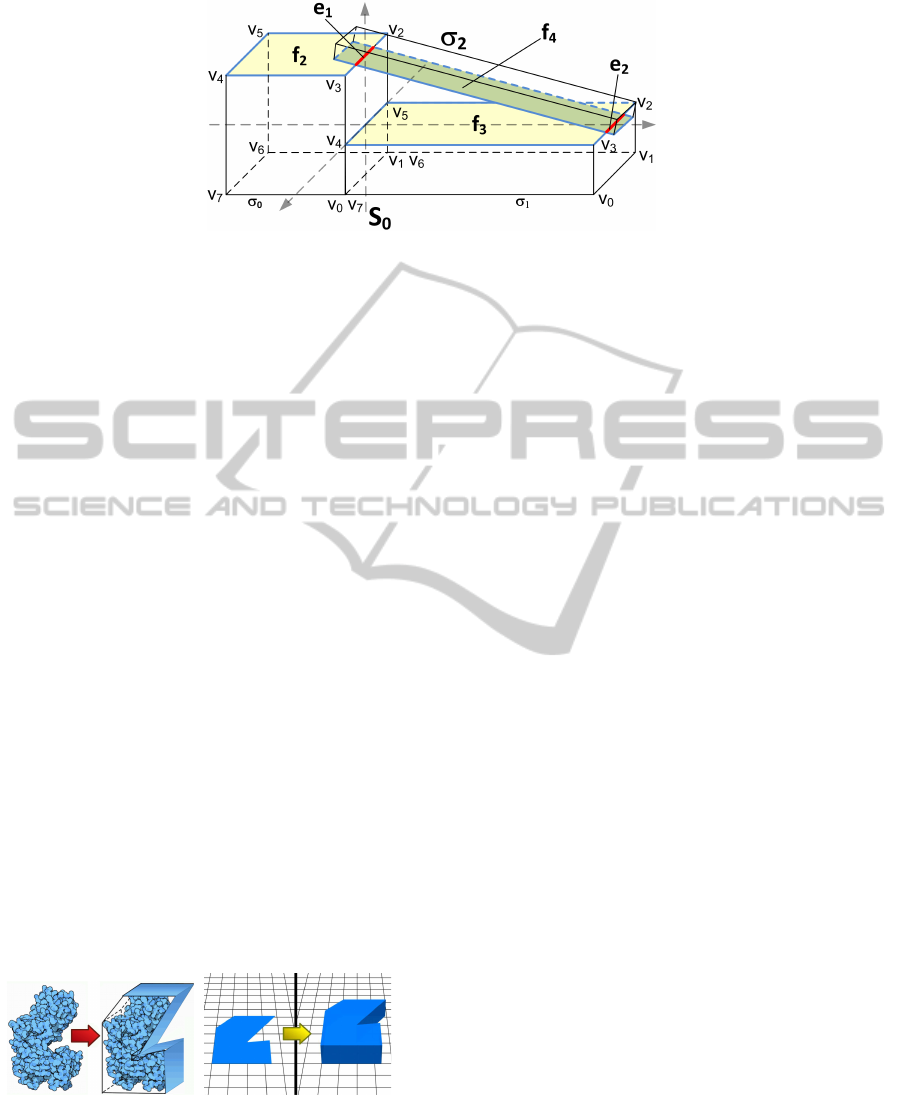
Figure 7: A compound 3D process, generated by glueing together a process with a compound shape (S
0
) and a process with
a simple shape (σ
2
), clashing on compatible channels. Supposed α the name of the channel, two possible bounds can be
created: ha, {s
0
.e
1
, s
2
. f
4
}i and ha, {s
1
.e
2
, s
2
. f
4
}i with s
0
and s
1
names of the basic shapes σ
0
and σ
1
components of shape
S
0
. With more than one contact point available (red), one is chosen non-deterministically as the binding surface.
the processes are going to bind on the edge s
0
.e
1
=
[s
0
.v
2
, s
0
.v
3
] of σ
0
, then the new compound 3D pro-
cess has the form: S
0
[B
0
]ha, s
0
.e
1
, s
2
. f
4
iσ
2
[B
1
] where
B
0
and B
1
are the behaviours after the binding oc-
curred.
6 IMPLEMENTATION
The current implementation of BIOSHAPE takes
as input an XML file containing the specification
of the shapes, the behaviours associated and other
simulation-related information. The related XML
Schema provides the right means to declare vertices
and faces according to the IFS representation de-
scribed in Section 4.
It can be argued that such representation is quite
tedious to be defined by hand and also difficult to un-
derstand at first glance (cfr. Figure 4(b)), discourag-
ing a potential user. However, in the 3D simulation
field, several different approaches have been proposed
to alleviate this issue simply by making the generation
of the actual coordinate points and faces transparent
to the user. Among others, the inflatable icons ap-
proach (Repenning, 2005) seems the most suitable to
be implemented in BIOSHAPE (Buti et al., 2011a).
(a) (b)
Figure 8: An hexokinase enzyme can be approximated to a
concave polyhedral shape (a). The same polyhedral shape
can be generated through inflation (b).
In the inflatable icons technique the user draws a
simple 2D form of the final shape and then inflates it
in order to create a 3D form (see Figure 8 for an exam-
ple). Inflation can be applied with different strengths
to different portions of the 2D/3D entity, to create par-
ticularly complex (still polyhedral) shapes. Note that
the user can generate even non-convex shapes, such
as the approximated hexokinase enzyme in Figure 8.
Suitable algorithms can be applied to calculate auto-
matically a convex decomposition of the shape, ei-
ther on the 2D representation — see (Keil, 2000) for
several approaches — or on the final 3D one — see
(Belov, 2002).
7 CONCLUSIONS
The Shape Calculus provides a power syntax and se-
mantics to model (not only) biological processes with
particular regard to the spatial aspects. In this pa-
per we refined the language to provide a more de-
tailed, finitary, geometric representation of shapes and
their communication channels. The resulting lan-
guage maintains the same characteristics of the origi-
nal one, adding a simple, yet powerful, way to define
and manage geometry. Differently from the original
characterization the newer syntax permits to directly
embed a Shape Calculus model into a simulation in
BIOSHAPE and still verification techniques can be
applied. To give more evidence on this, the refine-
ment proposed in this work can be re-formulated in
the Abstract Interpretation (Cousot and Cousot, 1977)
framework. We leave this as future work.
REFERENCES
Aleksandrov, A. D. (2005). Convex polyhedra. Springer
monographs in mathematics. Springer.
Baraff, D. (1997). An introduction to physically based
modeling: Rigid body simulation i - unconstrained
SIMULTECH2012-2ndInternationalConferenceonSimulationandModelingMethodologies,Technologiesand
Applications
226

rigid body dynamics. In An Introduction to Physi-
cally Based Modelling, SIGGRAPH ’97 Course Notes,
page 97.
Bartocci, E., Cacciagrano, D. R., Berardini, M. R. D.,
Merelli, E., and Tesei, L. (2010a). Timed operational
semantics and well-formedness of shape calculus. Sci.
Ann. Comp. Sci., 20:32–52.
Bartocci, E., Corradini, F., Berardini, M. R. D., Merelli, E.,
and Tesei, L. (2010b). Shape calculus. a spatial mobile
calculus for 3d shapes. Sci. Ann. Comp. Sci., 20:1–31.
Belov, G. (2002). A modified algorithm for convex
decomposition of 3d polyhedra. Technical Re-
port MATH-NM-03-2002, Institut f
¨
ur Numerische
Mathematik,Technische Universit
¨
at, Dresden.
http://www.math.tu-dresden.de/ belov/cd3/cd3.ps.
Buti, F., Cacciagrano, D. R., Callisto De Donato, M., Corra-
dini, F., Merelli, E., and Tesei, L. (2011a). Bioshape:
End-user development for simulating biological sys-
tems. In Costabile, M., Dittrich, Y., Fischer, G., and
Piccinno, A., editors, End-User Development, volume
6654 of Lecture Notes in Computer Science, pages
379–382. Springer Berlin / Heidelberg. 10.1007/978-
3-642-21530-8 45.
Buti, F., Cacciagrano, D. R., Corradini, F., Merelli, E., and
Tesei, L. (2010a). BioShape: a spatial shape-based
scale-independent simulation environment for biolog-
ical systems. Procedia Computer Science, 1(1):827–
835. Proc. of 7th Int. Workshop on Multiphysics Mul-
tiscale Systems, ICCS 2010.
Buti, F., Cacciagrano, D. R., Corradini, F., Merelli, E., and
Tesei, L. (To appear 2011b). A uniform multiscale
meta-model of BioShape. Electronic Notes in Theo-
retical Computer Science. Proc. of Cs2Bio 2011, June
9th, Reykjavik, Iceland.
Buti, F., Cacciagrano, D. R., Corradini, F., Merelli, E., Te-
sei, L., and Pani, M. (2010b). Bone Remodelling in
BioShape. Electronic Notes in Theoretical Computer
Science, 268:17–29. Proc. of CS2Bio 2010.
Corradini, F. and Merelli, E. (2005). Hermes: Agent-based
middleware for mobile computing. In Bernardo, M.
and Bogliolo, A., editors, Formal Methods for Mobile
Computing, volume 3465 of Lecture Notes in Com-
puter Science, pages 234–270. Springer Berlin / Hei-
delberg.
Cousot, P. and Cousot, R. (1977). Abstract interpretation:
a unified lattice model for static analysis of programs
by construction or approximation of fixpoints. In In
Proc. of POPL’77, pages 238–252. ACM.
Ericson, C. (2005). Real-time collision detection. Num-
ber v. 1 in Morgan Kaufmann Series in Interactive 3D
Technology. Elsevier.
Ferrari, M. (2005). Cancer nanotechnology: opportunities
and challenges. Nature Reviews Cancer, 5(3):161–
171.
Grupe, A., Germer, S., Usuka, J., Aud, D., Belknap, J. K.,
Klein, R. F., Ahluwalia, M. K., Higuchi, R., and Peltz,
G. (2001). In Silico Mapping of Complex Disease-
Related Traits in Mice. Science, 292(5523):1915–
1918.
Hartman, J. and Wernecke, J. (1996). The VRML 2.0 hand-
book: building moving worlds on the web. Addison
Wesley Longman Publishing Co., Inc., Redwood City,
CA, USA.
Hoffmann, C. M. (1989). Geometric and solid modeling: an
introduction. Morgan Kaufmann series in computer
graphics and geometric modeling. Morgan Kaufmann.
Kawasaki, E. S. and Player, A. (2005). Nanotechnology,
nanomedicine, and the development of new, effective
therapies for cancer. Nanomedicine: Nanotechnology,
Biology and Medicine, 1(2):101 – 109.
Keil, J. M. (2000). Polygon decomposition. In Sack, J.
and Urrutia, J., editors, Handbook of Computational
Geometry, pages 491–518. Elsevier.
Kitano, H. (2002). Systems biology: a brief overview. Sci-
ence, 295(5560):1662–1664.
Kumar, C. S. S. R. (2007). Nanomaterials for medical di-
agnosis and therapy. Nanotechnologies for the life
sciences. Wiley-VCH.
Lim, H. A. (2004). Nanotechnology in diagnostics and
drug delivery. Medicinal Chemistry Research, 13(6-
7):401–413.
Manos, S., Zasada, S., and Coveney, P. V. (2008). Life or
Death Decision-making: The Medical Case for Large-
scale, On-demand Grid Computing. CTWatch Quar-
terly, 4(1).
M
¨
antyl
¨
a, M. (1988). An Introduction to Solid Modeling.
Computer Science Press, College Park, MD.
Milner, R. (1982). A Calculus of Communicating Systems.
Springer-Verlag New York, Inc., Secaucus, NJ, USA.
Minton, A. P. (1998). Molecular crowding: Analysis of ef-
fects of high concentrations of inert cosolutes on bio-
chemical equilibria and rates in terms of volume ex-
clusion. In Gary K. Ackers, M. L. J., editor, Energetics
of Biological Macromolecules Part B, volume 295 of
Methods in Enzymology, pages 127 – 149. Academic
Press.
Mirtich, B. (1998). V-clip: fast and robust polyhedral colli-
sion detection. ACM Trans. Graph., 17:177–208.
Murray, J. D. and VanRyper, W. (1996). Encyclopedia of
graphics file formats. O’Reilly Series. O’Reilly & As-
sociates.
Repenning, A. (2005). Inflatable icons: Diffusion-based in-
teractive extrusion of 2d images into 3d models. Jour-
nal of Graphics, Gpu, and Game Tools, 10(1):1–15.
Takahashi, K., Arjunan, S. N. V., and Tomita, M. (2005).
Space in systems biology of signaling pathways–
towards intracellular molecular crowding in silico.
FEBS letters, 579(8):1783–1788.
Taylor, C. A., Draney, M. T., Ku, J. P., Parker, D., Steele,
B. N., Wang, K., and Zarins, C. K. (1999). Biomedical
paper predictive medicine: Computational techniques
in therapeutic decision-making.
Torchilin, V. P. (2006). Nanoparticulates as drug carriers.
Imperial College Press.
Van den Berg, B., Ellis, R. J., and Dobson, C. M. (1999).
Effects of macromolecular crowding on protein fold-
ing and aggregation. The European Molecular Biol-
ogy Organization Journal, 18(24):6927–6933.
AGeometricalRefinementofShapeCalculusEnablingDirectSimulation
227
