
A Simple Efficient Technique to Adjust Time Step Size
in a Stochastic Discrete Time Agent-based Simulation
Chia-Tung Kuo, Da-Wei Wang and Tsan-sheng Hsu
Institute of Information Science, Academia Sinica, Taipei, Taiwan
Keywords:
Simulation, Step Size, Efficiency, Granularity.
Abstract:
This paper presents a conceptually simple approach on adjusting the time step size in a stochastic discrete time
agent-based simulation and demonstrates how this could be done in practical implementation. The choice of
time step size in such a system is often based on the nature of the phenomenon to be modelled and the
tolerated simulation time. A finer time scale may be desired upon the introduction of new events which
could possibly change the system state in smaller time intervals. Our approach divides each original time
step into any integral number of equally spaced sub-steps based on simple assumptions, and thus allows a
simulation system to incorporate such events and produce results with finer time scale. Regarding the trade-
off between finer scale and higher use of resource, our approach also highlights the implementation techniques
that increase the resource usage and simulation time only marginally. We analyze the results of this refinement
on a stochastic simulation model for epidemic spread and compare the results with the original system without
refinement.
1 INTRODUCTION
The stochastic discrete time simulation model is a
useful and efficient way in simulating agent-based ac-
tivities and has gained significant popularity in mod-
elling many dynamical biological or physical sys-
tems in recent years, such as the dynamics of epi-
demic spread (Tsai et al., 2010a; Riley, 2007). Often
time, such simulations can give insights into problems
where traditional models are too complicated and an-
alytic results are very difficult or currently impossible
to obtain (Tsai et al., 2010a; Germann et al., 2006).
This high level abstraction, however, introduces ar-
tifacts which do not pertain to real world behaviour,
namely, the discretization of time. In particular, event
simultaneity whereby multiple distinct events occur
at exactly the same time may be due to an insuf-
ficiently detailed discrete-time model (Vangheluwe,
2001). The additional parameter, the size of the
time step, can potentially have significant impact on
the results of simulation without the awareness of
the modeller (Buss and Rowaei, 2010). Buss and
Rowaei investigated time advancement mechanism
and the role of time step size in a somewhat different
context (Buss and Rowaei, 2010; Buss and Rowaei,
2011), and found no systematic studies had been done
with its effects. Moreover, the choice of time step si-
ze plays a role in the efficiency of the simulation as
the occurrence of events need to be checked more fre-
quently for smaller time steps. Accordingly, the size
of the time step should be carefully selected to match
the real world phenomenon to be modelled as real-
istically as possible, and without too much sacrifice
of simulation time. Other than for its realistic nature,
this choice of time step size is often influenced by the
empirical data we have. For example, in modelling
the epidemic spread, the unit of measurements for la-
tent and infectious periods also affect the choice of
time step size (Kelker, 1973). Specifically, the unit of
measurements for latent and infectious periods should
be smaller than or equal to the length of a time step
to make sure that no event advances two steps in one
simulated time step.
We have developed a simple, yet efficient, tech-
nique based on reasonable assumptions to split each
time step into any integral number of equally spaced
sub-steps with small increase in simulation time in a
stochastic discrete time agent based simulation sys-
tem for epidemic spread we developed earlier (Tsai
et al., 2010a; Tsai et al., 2010b). More precisely,
we first modify the probabilities of events according
to the basic probability theory such that they corre-
spond to events occurring in a smaller time frame.
This allows the introduction of certain types of events
42
Kuo C., Wang D. and Hsu T..
A Simple Efficient Technique to Adjust Time Step Size in a Stochastic Discrete Time Agent-based Simulation.
DOI: 10.5220/0004056000420048
In Proceedings of the 2nd International Conference on Simulation and Modeling Methodologies, Technologies and Applications (SIMULTECH-2012),
pages 42-48
ISBN: 978-989-8565-20-4
Copyright
c
2012 SCITEPRESS (Science and Technology Publications, Lda.)

in a smaller time scale. Then we introduce a struc-
turally different implementation model that signifi-
cantly outperforms the straightforward step-by-step
linear model. The experiments show that our im-
proved implementation produces stochastically iden-
tical results as the straightforward implementation
with significantly less time. Furthermore, our results
also show that, given the same set of possible events,
simulation with a finer time scale causes events to oc-
cur slightly earlier. This is well justified since we as-
sign certain probability of occurrence to each event
in a smaller time interval and update the system state
more frequently.
This paper is organized as follows. Section 2 gives
a simplified view of the basic model of a stochastic
discrete time agent-based simulation. Section 3 de-
scribes our adjustment and its implementation. Sec-
tion 4 demonstrates our experimental results and pro-
vides a discussion of these results. Section 5 de-
scribes the general applicability of our approach and
discusses its limitations. Section 6 concludes our pa-
per and points out directions for future work.
2 SIMULATION MODEL
In this section, we describe the basic model of a
stochastic discrete time agent-based simulation sys-
tem, with specific reference to the simulation system
developed by (Tsai et al., 2010a) following approach
in (Germann et al., 2006). Algorithm 1 provides a
high level description of the agent-based simulation
model of an epidemic spread.
Algorithm 1: Stochastic agent-based simulation model.
1: for each time step T from beginning to
end of simulation do
2: for each infectious agent I do
3: for each susceptible agent S in contact
with I during T do
4: if I infects S successfully then
5: update status of S
6: end if
7: end for
8: end for
9: end for
The time step refers to the indexing variable in
the outermost loop. This step size characterizes the
unit of time in which the system progresses. In other
words, the system state must remain constant between
successive steps; thus, all events must occur with pe-
riods of integral multiples of this time step size. In
line 2, we identify the agents that may change the sys-
tem state in the current time step. In the inner loop, for
each of these agents, we find all interacting agents in
the same step, and decide whether an event between
agents actually occurs. There are often times sched-
uled events other than among interacting agents that
may take place; these could be dealt with similarly
and we focus our attention on events described in Al-
gorithm 1.
In our simulation of an epidemic spread, each time
step is one half-day. This is largely due to the facts
that agents (people) are in contact with different other
agents during daytime and nighttime, and also state
transitions take place in multiple of half-days. An
agent is classified as one of the susceptible, infec-
tious, and recovered (or removed); in each step, an
infectious agent may infect susceptible agents in con-
tact according to a transmission probability, which is
dependent upon the interacting agents’ ages and con-
tact locations. Once an infectious agent successfully
infects a susceptible agent, the susceptible will be as-
signed a latent period and an infectious period, and
become infectious at the end of the half-day step.
These latent and infectious periods are drawn from
two pre-specified discrete random variables, derived
from observed data on the epidemic to be modelled.
Besides the obvious possibility where finer time
scale result is desired, there are still at least two poten-
tial issues with this current model regarding the size
of the time step. First, if we wish to model a dis-
ease for which the latent and infectious periods are
better modelled with finer time unit, the current sys-
tem could not easily accommodate this change with-
out major revision efforts. Second, if we wish to (in-
deed we do) record not only who is infected, but also
the infector, then the artificial simultaneity (See Sec-
tion 1) may be introduced: two or more infectious
nodes may infect the same susceptible agent in one
step, and thus some mechanism is required to decide
the infector precisely.
In the next section, we introduce a modified
model, which is the same as the original model in
principle but divides each step into integral number
of smaller sub-steps. In section 3.2, we describe effi-
cient techniques in implementation that could achieve
our desired results with minimal increase in simula-
tion time.
ASimpleEfficientTechniquetoAdjustTimeStepSizeinaStochasticDiscreteTimeAgent-basedSimulation
43

3 ADJUSTMENT OF TIME STEP
SIZE
3.1 Finer Step Model
In the original model, each pair of infectious (I) and
susceptible (S) in contact are associated with a trans-
mission probability P
IS
. In each half-day step, we it-
erate through all pairs of infectious and susceptible
in contact, and for each pair, decide whether S is in-
fected by I with probability P
IS
. Now, for each P
IS
,
we derive a k-hour transmission probability, p
IS
k
, that
satisfies
(1 − p
IS
k
)
12
k
= 1 − P
IS
(1)
where k is a factor of 12 (we use the term, granular-
ity of the system, to denote the smallest unit of time
interval in which an event to be modelled could take
place). The probability p
IS
k
is derived such that the
overall probability of S getting infected by I does not
change if S is decided for infection with probability
p
IS
k
every k hour(s), provided that no change in state
occurs in each half-day step. Notice that this deriva-
tion also makes the assumptions that the probability
of transmitting a disease is uniform in the half-day
step and independent among each smaller sub-steps.
That is, we use the same p
IS
k
for all sub-steps, in-
stead of a number of different (conditional) probabili-
ties. These may be debatable assumptions, depending
upon what events are being modelled.
The probability p
IS
k
is derived between each IS-
pair; we would like the probabilities of transmitting
a disease (between any pair) in each step to be the
same as the original probability, P
IS
in cases of mul-
tiple pairs of infectious and susceptible agents in con-
tact. Now we show that this is indeed the case. More
formally, the probability of each susceptible agent S
getting infected remains the same as long as the du-
ration of contact between each IS-pair is unchanged
and a multiple of 12-hour. Notice that it suffices to
demonstrate the case where there are more than one
infectious agents in contact with only one suscepti-
ble agent, as susceptible agents do not influence each
other. This is an immediate result from the assumed
independence of infection events by different infec-
tious agents and the commutative property of mul-
tiplication. Suppose there are n infectious agents,
I
1
,...,I
n
and one susceptible agent S in contact in some
arbitrary half-day step. Let S
t
and S
t
denote the events
S gets infected at t and S gets infected by t, respec-
tively. Also, we use ¬ to denote logical negation.
Then,
Pr{S infected} = 1 − Pr{S not infected}
= 1 − Π
12
t
j
= jk, j∈N
Pr{¬S
t
j
|¬S
t
j−1
}
= 1 − Π
12
t
j
= jk j∈N
Π
n
i=1
Pr{¬S
t
j
by I
i
|¬S
t
j−1
}
= 1 − Π
n
i=1
Π
12
t
j
= jk, j∈N
(1 − p
I
i
S
k
)
= 1 − Π
n
i=1
(1 − P
I
i
S
)
Notice that in the derivation above, we split one half-
day into 12/k sub-steps of k hour(s) each. The same
approach could be used for splitting a time step of any
size into any integral number of equally spaced sub-
steps.
This refinement does not introduce any conceptu-
ally new artefact into the model. All it does is to per-
form the simulation with shorter time step size, and
in each time step, the probabilities for events to occur
are altered. Specifically, in Algorithm 1, we substitute
a step with a smaller sub-step in the outermost loop,
and use p
IS
k
instead of P
IS
when deciding infection
(line 4). Regarding the two concerns we have at the
end section 2, the first is solved as we can now model
any events that take place with periods greater than
or equal to the granularity of the system (k hours in
this example). This approach does not deal with the
second concern directly. However, by reducing the
time step size (and thus the transmission probability
in a step), the chances of simultaneous events could
be reduced significantly.
Now a new issue concerning efficiency is intro-
duced. Typically, in a large scale agent-based sim-
ulation system, the number of possible interactions
among agents or other events (line 2 in Algorithm 1)
is very large in each step. Therefore, after applying
this technique to reduce the step size, we will exam-
ine, in each step, a long list of possible events, of
which most will not take place due to the reduced
probabilities. In response to this efficiency issue, in
section 3.2 we introduce techniques in implementa-
tion, which allow the system to run almost as fast as
with the coarser time step, but achieve the benefits
produced by the finer time step.
3.2 Efficient Implementation
Our goal in this section is to implement the refined
model more efficiently. For the ease of description,
we refer to the original time step (e.g. half-day in
the model above) as step, and the finer time step (e.g.
k hour(s)) as sub-step, and also maintain the use of P
and p
k
to denote the transmission probabilities in each
step and sub-step, respectively. The challenge is that
we wish to achieve the effect of advancing the sys-
tem every sub-step unit of time, but we do not want
to examine all possible transmission events such fre-
SIMULTECH2012-2ndInternationalConferenceonSimulationandModelingMethodologies,Technologiesand
Applications
44
generate
random r
r < p
IS
k
?
infected at t
s
generate
random r
r < p
IS
k
?
infected
at t
s+1
.
.
.
.
.
.
infected at t
e
uninfected
yes
no
yes
no
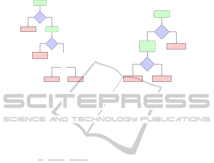
(a) Infection decision process sub-step
by sub-step.
generate
random r
r < P
IS
?
uninfected
select
i from
{0,1,. . . ,α}
s + i ≤ e
infected at t
s+i
uninfected
yes
no
yes
no
(b) Infection decision process in our
refined implementation.
Figure 1: Schematic pictures of infection decision processes for an IS-pair in one full step T ; step T consists of sub-steps t
1
,
t
2
, ..., t
α
, and I starts infecting at t
s
∈ T and recovers at t
e
∈ T where t
e
is later than t
s
. Notice that in both (a) and (b), r is
drawn uniformly random from (0,1), while in (b) i is drawn from the computed distribution accordingly.
quently. The main idea here is to make the ”big de-
cision” first, and make subsequent ”small decisions”
only if the first result turns out ”favorable”. First, we
”select” a possible transmission event with the aggre-
gate probability, P
IS
. This determines whether this
agent gets infected in a step. Following that, we de-
cide which sub-step this event actually occurs accord-
ing to probabilities,
p
IS
k
P
IS
,
p
IS
k
(1−p
IS
k
)
P
IS
,
p
IS
k
(1−p
IS
k
)
2
P
IS
, ....
Flow charts of infection decisions between an IS-pair
are shown in Figure 1.
From Figure 1, it is straightforward to verify that
in our modified implementation, the probability of an
infectious agent transmitting the disease to a suscep-
tible agent in contact in a step is the same as in the
original model. In cases of multiple IS-pairs, an ar-
gument similar to the one in Section 3.1 could show
that the probabilities of transmission do not change,
provided the length of duration for any IS-pair in con-
tact is fixed. There is, however, one more premise
for this implementation to work: the contacts among
agents in a step must be known before we start the
step. This is necessary since we iterate through in-
fectious agents only every step , instead of every sub-
step as in Section 3.1. This assumption is often easily
satisfied as in many agent-based simulations, the pos-
sible interactions among agents are determined by the
pre-initialized properties of the agents (e.g. the con-
tact locations in which agents reside).
The argument above shows that this improved im-
plementation should, in principle, achieve the same
result as the straightforward sub-step by sub-step im-
plementation (Algorithm 1). However, we point out
three issues (may be more for more complicated mod-
els) for which extra care should be taken in practical
implementation, in order to get this expected result:
1. Notice in the actual model with period being a
sub-step, an event may become ready or may be
removed between two successive sub-steps within
a step. For example, in the model of epidemic
spread, an infectious agent I may recover, or a
susceptible agent S may turn infectious in any
sub-step, so that contact with I no longer results
in new infections, or new transmission routes be-
come possible within a step. In these cases, as-
suming the knowledge of when events are ready or
removed is known before each step, we can per-
form a simple lookup and filter out those events
that we have determined its occurrence in a sub-
step before it is ready or after it has been removed.
2. It is possible that two events could each occur with
some probabilities, but they could not occur both
in the same sub-step. That is, the occurrence of
one prevents the occurrence of the other one. This
issue pertains to the problem of ”artificial simul-
taneity” in section 1 where some arbitrary order-
ing is needed. For example, a susceptible agent S
cannot get infected from two infectious agents I
1
and I
2
in two different sub-steps of the same step.
To conform to the original model (Algorithm 1)
with time period being a sub-step, we must ig-
nore the occurrence of all conflicting events in a
step except the one which occurs in the earliest
sub-step (There could still be more than one oc-
curring in the earliest sub-step; in this case, an ar-
ASimpleEfficientTechniquetoAdjustTimeStepSizeinaStochasticDiscreteTimeAgent-basedSimulation
45

bitrary selection is made. But the chances of such
cases are significantly reduced as indicated in sec-
tion 3.1).
3. The occurrence of an event in a sub-step may
introduce new events that are possible to occur
immediately starting from the next sub-step. To
deal with these cases, a list of these possible new
events must be maintained in a step, and each
event in this list is to be decided for its occur-
rence and cleared in the current step. This it-
erative examination will eventually terminate as
fewer events will be added for the remaining sub-
steps and probabilities of occurrence are smaller
as well. If a later examined event A takes place
and prevents the occurrence of an earlier decided
event B , which occurs later than A in time (as
illustrated in issue 2), we must update the sys-
tem accordingly to take event A and ignore event
B. For example, consider the case where in some
step T, an infectious agent I
1
successfully infects
a susceptible agent S
1
at sub-step t
1
and another
susceptible agent S
2
at a later sub-step t
2
(t
1
< t
2
,
but they belong to the same step T ). Assume S
1
turns infectious immediately and successfully in-
fects S
2
in sub-step t
3
where t
1
< t
3
< t
2
. Then
we must update the infection time of S
2
to be t
3
in stead of t
2
. In practical implementation, the list
of these newly triggered events within the same
step should be sorted in order of the sub-steps of
occurrence to avoid a long sequence of updates in
the cases of the example above.
Algorithm 2 gives a high-level description of the
practical implementation of the system that could
achieve the same results as in Algorithm 1 with finer
step size.
4 EXPERIMENTAL RESULTS
AND DISCUSSION
In this section, we wish to demonstrate that our re-
fined model indeed achieves stochastically identical
results as the original model with a shorter time pe-
riod, and significantly reduces the simulation time.
Also, we give a reasonable account for the observed
differences in results from simulations of different
time step sizes.
We build the two simulation systems (denoted by
ALG
1
and ALG
2
for Algorithm 1 and Algorithm 2, re-
spectively) by modifying a simulation system for epi-
demic spread developed by (Tsai et al., 2010a), keep-
ing all parameters as original except the ones we ex-
plicitly wish to manipulate. Below, we perform 100
Algorithm 2: Refined stochastic agent-based simulation
model.
1: for each time step T from beginning to
end of simulation do
2: initialize an empty sorted list L =
/
0
3: for each infectious agent I do
4: TryToInfect (I, T,L )
5: end for
6: while L is not empty do
7: I
new
← remove the head of L
8: TryToInfect (I
new
,T, L )
9: end while
10: end for
11: procedure TRYTOINFECT(I,T ,L )
12: for each susceptible agent S in contact with I
during T do
13: if I is still infectious and infects S success-
fully in sub-step t, and S has not been infected
before t then
14: update status of S
15: if S turns infectious within the current
step T then
16: Add S to L
17: end if
18: end if
19: end for
20: end procedure
baseline simulations for each system with a particular
granularity, and report the average results for both the
simulation outputs and the simulation time consumed.
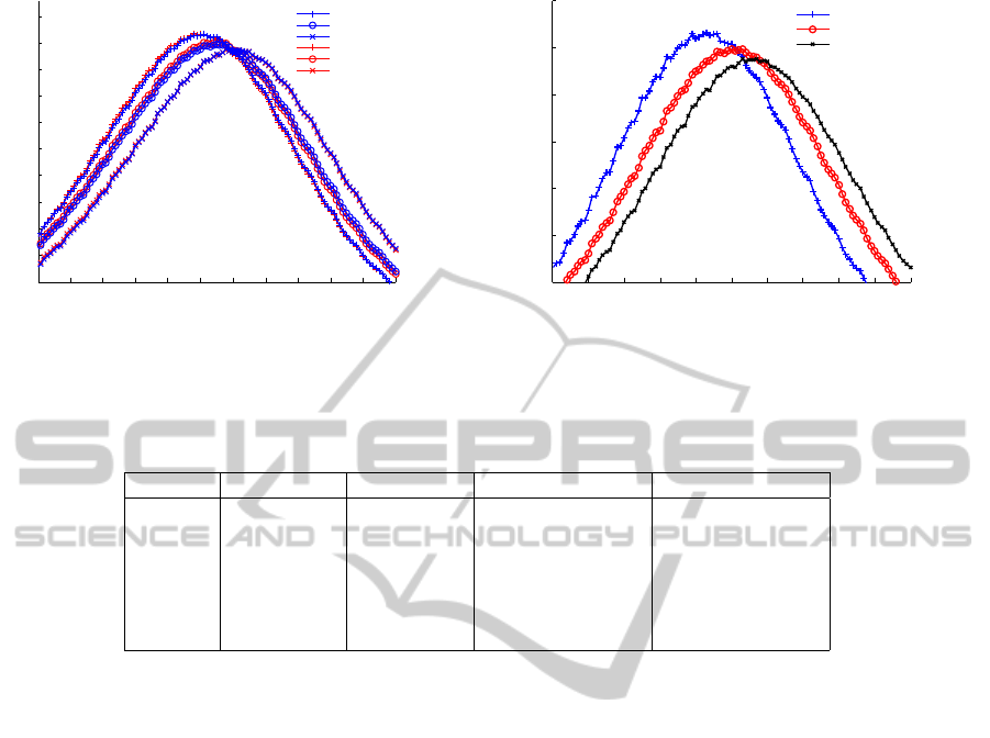
Figure 2(a) shows the epidemic curves (daily new
cases) produced by the two systems, ALG
1
(blue) and
ALG
2
(red), when granularity (GR) is set to 1 (+),
6 (o), and 12 (x) hour(s), respectively. Each pair of
curves corresponding to the same granularity over-
lap well, showing that this modified implementation
indeed reproduces the result of the original model.
Moreover, the leftward shift of epidemic curves for
finer granularities is also expected. This is a result
of our assumption that the probability of transmission
in each smaller step is uniformly distributed, and this
causes the expectation of infection time to become
earlier. Similar phenomenon is also observed if we
shorten the latent period since it does not affect infec-
tivity while causing a earlier spread of disease. Fig-
ure 2(b) shows the epidemic curves produced by the
original system with varied latent periods.
Table 1 shows the average simulation times (Sim-
Time in seconds) and attack rates (AR) for each of the
two systems run on a workstation with 8 Intel Xeon
X5365 CPUs and 32GB RAM. The consistency in at-
SIMULTECH2012-2ndInternationalConferenceonSimulationandModelingMethodologies,Technologiesand
Applications
46
130 140 150 160 170 180 190 200 210 220 230 240
1
1.5
2
2.5
3
3.5
4
4.5
5
5.5
6
x 10
4
Day
Daily new cases
ALG1 GR=1
ALG1 GR=6
ALG1 GR=12
ALG2 GR=1
ALG2 GR=6
ALG2 GR=12
(a) Epidemic curves by ALG
1
and ALG
2
with different
granularities.
100 110 120 130 140 150 160 170 180 190 200
2
3
4
5
6
7
8
x 10
4
Day
Daily new cases
short latent
medium latent
long latent
(b) Epidemic curves for different lengths of latent peri-
ods.
Figure 2: Average epidemic curves from 100 simulations.
Table 1: Average attack rates and simulation times for the two systems ALG
1
and ALG
2
with different granularities.
GR (hr) AR (ALG
1
) AR (ALG
2
) SimTime (ALG
1
) SimTime (ALG
2
)
1 0.312 0.312 971 134
2 0.312 0.312 504 133
3 0.312 0.312 351 133
4 0.312 0.312 276 133
6 0.312 0.312 203 133
12 0.311 0.311 127 130
tack rates confirms our argument that the overall prob-
abilities of infection are not altered; the huge reduc-
tion in simulation time demonstrates the effectiveness
of our proposed model for practical implementation.
5 APPLICABILITY AND
LIMITATIONS
We briefly describe the context in which this approach
is applicable, as well as its current limitations. This
approach was initially designed to handle situations
in epidemic spread where we want a disease’s natural
history that is finer than the time step size in the origi-
nal model. This was achieved by certain assumptions
and basic probability theory, as shown in section 2.
Algorithm 2 was then developed to improve the ef-
ficiency of the straightforward model (Algorithm 1)
with a small step size and small interacting probabil-
ities among agents. As a result, it should be easily
applicable to other agent-based simulations when a
similar factor affecting agents’ interactions needs to
be measured in finer time scale; that is agents could
become active (e.g. infectious) or inactive (e.g. re-
covered or isolated) in such time scale.
It is crucial to notice that the sub-step in which
agents become inactive must be known before the
start of each step (the case of turning activein the mid-
dle of a step could be handled as described in section
3.2 issue 3). It is not a problem in our example of
epidemic spread simulation as the length of latent and
infectious periods of an agent (thus the information of
when it recovers) is determined when the agent gets
infected. This, however, may pose a problem for other
kinds of simulations. It may require tracing back of
when an agent becomes inactive, and undoing all its
interactions thereafter.
6 CONCLUDING REMARKS AND
FUTURE WORK
We proposed a simple approach in adjusting the time
step size in a stochastic discrete time agent-based sim-
ulation model based on reasonable assumptions. This
provides flexibility in modelling events with finer
time scales; such flexibility is often desired when
finer empirical observations were to be incorporated
into simulations. Furthermore, we described a struc-
turally different model for practical implementation,
which achieves identical result significantly faster. To
demonstrate this, we modified a simulation system for
ASimpleEfficientTechniquetoAdjustTimeStepSizeinaStochasticDiscreteTimeAgent-basedSimulation
47

epidemic spread, developed by (Tsai et al., 2010a),
constructed the proposed simulation model in both
ways (Algorithm 1 and Algorithm 2), and through
experiments, showed that they indeed computed the
same results with the later one having a huge reduc-
tion in simulation time.
The implementation technique introduced in this
paper may also be applied to purely increase the ef-
ficiency without any effect on results; we could view
the original time step as the sub-step and run the sys-
tem with an enlarged step following Algorithm 2 to
produce the same result more efficiently. This may,
however, introduce difficulties in determining the pos-
sible events to occur in an enlarged step. In the ex-
ample of the epidemic spread simulation, two agents
may be in contact only in daytime and not nighttime
(see Algorithm 1 line 3); in an enlarged step, attention
must be paid to such circumstances. It is also likely
that other calibrated parameters need to be rescaled
appropriately when such refinement is employed. We
will work on overcoming the limitations mentioned
above and in section 5, and try to apply such tech-
niques to a larger variety of general simulations.
Another interesting direction is to compare the ef-
fect of time step size in discrete time agent-based sim-
ulations with the more traditional approaches to sim-
ulation modelling, such as event scheduling, and also
the modelling with differential equations, commonly
seen in mathematical epidemiology (Diekmann and
Heesterbeek, 2000).
ACKNOWLEDGEMENTS
We thank anonymous reviewers for their comments
and suggestions. Also we sincerely thank Steven
Riley (s.riley@imperial.ac.uk) for his valuable com-
ments throughout this study.
REFERENCES
Buss, A. and Rowaei, A. A. (2010). A comparison of the
accuracy of discrete event and discrete time. In Pro-
ceedings of the 2010 Winter Simulation Conference.
Buss, A. and Rowaei, A. A. (2011). The effects of time ad-
vance mechanism on simple agent behaviors in com-
bat simulations. In Proceedings of the 2011 Winter
Simulation Conference.
Diekmann, O. and Heesterbeek, J. (2000). Mathematical
Epidemiology of Infectious Diseases: Model Building,
Analysis, and Interpretation. John Wiley and Sons
Ltd.
Germann, T. C., Kadau, K., Ira M. Longini, J., and Macken,
C. A. (2006). Mitigation strategies for pandemic in-
fluenza in the united states. In Proceedings of the Na-
tional Academy of Sciences, volume 103, pages 5935–
5940.
Kelker, D. (1973). A random walk epidemic simula-
tion. Journal of the American Statistical Association,
68(344):821–823.
Riley, S. (2007). Large-scale spatial-transmission models
of infectious disease. Science, 316(5627):1298–1301.
Tsai, M.-T., Chern, T.-C., Chuang, J.-H., Hsueh, C.-W.,
Kuo, H.-S., Liau, C.-J., Riley, S., Shen, B.-J., Shen,
C.-H., Wang, D.-W., and Hsu, T.-S. (2010a). Efficient
simulation of the spatial transmission dynamics of in-
fluenza. PloS ONE.
Tsai, M.-T., Wang, D.-W., Liau, C.-J., and sheng Hsu, T.
(2010b). Heterogeneous subset sampling. In Lecture
Notes in Computer Science, volume 6196, pages 500–
509.
Vangheluwe, H. (2001). Discrete event modelling and sim-
ulation. Lecture Notes, CS522 McGill University.
SIMULTECH2012-2ndInternationalConferenceonSimulationandModelingMethodologies,Technologiesand
Applications
48
