
A Generic Approach for the Identification of Variability
Anilloy Frank and Eugen Brenner
Institute of Technical Informatics, Technische Universit
¨
at, Inffeldgasse 16, 8010 Graz, Austria
Keywords:
Design Tools, Embedded Systems, Feature Extraction, Software Reusability, Variability Management.
Abstract:
The automotive electrical/electronics (E/E) embedded software development largely uses Model Based Soft-
ware Engineering (MBSE), an industrially accepted approach. With an ever increasing complexity of embed-
ded software, the E/E models in automotive applications are getting enormously unmanageable. The heteroge-
neous nature of projects developed using several modeling and simulation tools, and the hierarchical structure
with numerous composite components deeply embedded within, tends to repeatability. Hence it is often nec-
essary to define a mechanism to identify reusable components from these that are embedded deep within. The
proposed approach addresses the identification process in the development and deployment of software com-
ponents used in the realization of such distributed processes, by selectively targeting the component-feature
model (CF) instead of a comprehensive search to improve the identification. It addresses the issues to identify
commonality of variants within a product development. The results obtained are faster and are more accurate
compared to other methods.
1 INTRODUCTION
The current development trend in automotive soft-
ware is to map embedded software components on
networked Electronic Control Units (ECU) (Kum
et al., 2008).
Variants of embedded software functions are in-
evitable in customizing for different regions (Europe,
Asia, etc.), to meet regulations of the respective re-
gions. Also different sensors / actuators, different de-
vice drivers, and distribution of functionality on dif-
ferent ECUs necessitate variants (Frank and Brenner,
2010a); (Frank and Brenner, 2010b).
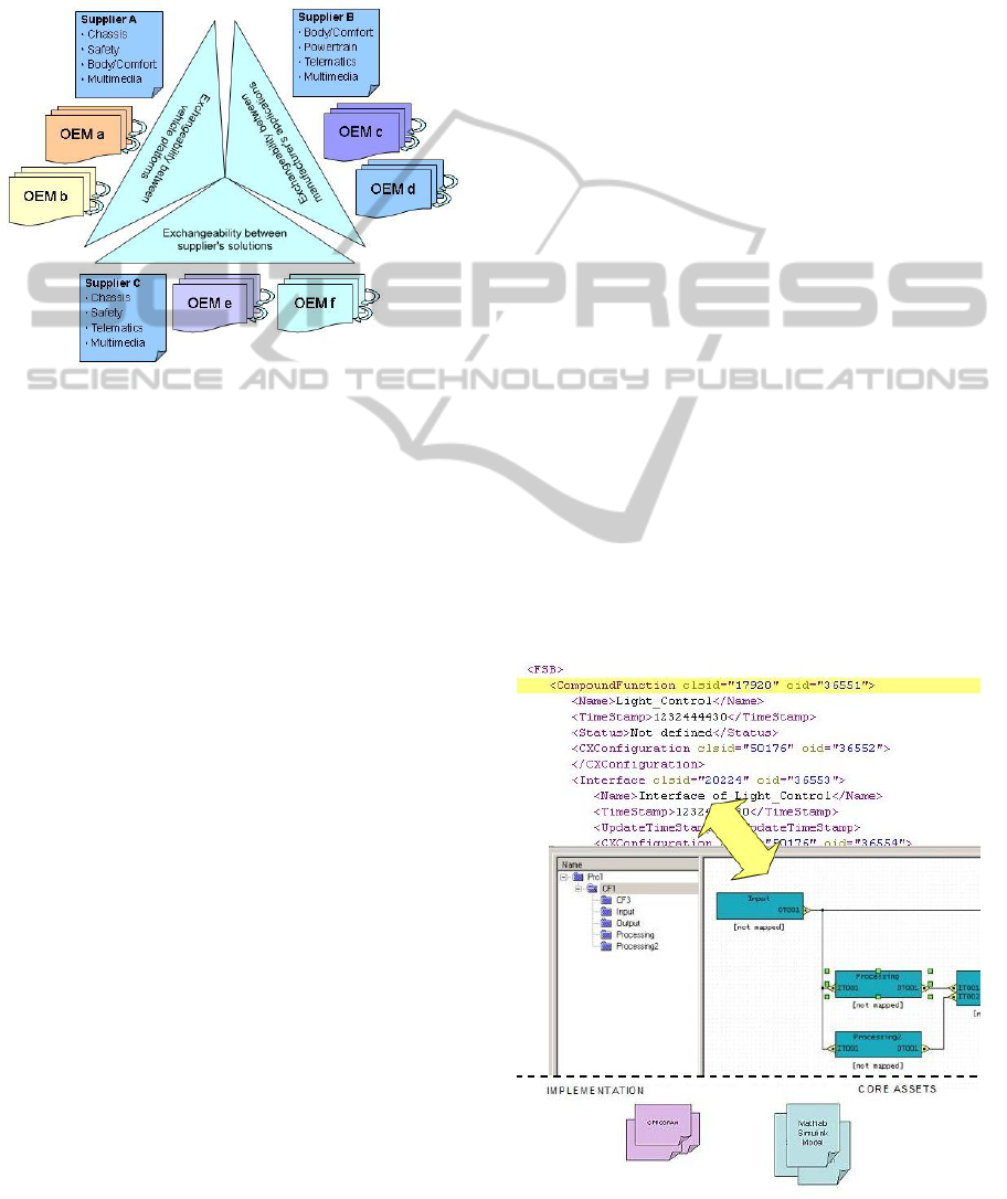
Often it is apparent to procure well established
software components tested for performance, safety
and reliability from external sources or Original
Equipment Manufacturers (OEM), illustrated in Fig-
ure 1. The black box characteristics of such software
components, when integrated in models, further add
to the complexity, and work as hindrance in manag-
ing variability.
Managing variability involves extremely complex
and challenging tasks, which must be supported by ef-
fective methods, techniques, and tools (Clements and
Northrop, 2007). In view of this complexity, achiev-
ing the required reliability and performance is one of
the most challenging problems (Bosch, 2000).
The proposed strategy is a model-based approach
for the distributed business process. The approach
intends to facilitate automated and interactive strate-
gies to addresses the identification process in the de-
velopment and deployment of software components.
We start by analyzing the textual representation of the
model structure and form a concept to extract an el-
ement list to facilitate the identification of variabil-
ity. Based on the adaptation of a formal mathematical
model presented in this paper is the implementation
and evaluation of the proposed strategy.
2 RELATED WORK
For achieving large-scale software reuse, reliability,
performance and rapid development of new products,
Software Product-Line Engineering(SPLE) is an ef-
fective strategy. SPLE can be categorized into domain
engineering and application engineering (Bachmann
and Clements, 2005); (Bosch, 2000). Domain en-
gineering involves design, analysis and implementa-
tion of core objects, whereas application engineering
is reusing these objects for product development.
Model Driven Software Development (MDSD) is
typically realized in a distributed system environment
for the development of automotive applications and
products (Kulesza et al., 2007). Model-based tech-
niques are used to support the usage of platform inde-
167
Frank A. and Brenner E..
A Generic Approach for the Identification of Variability.
DOI: 10.5220/0004009301670172
In Proceedings of the 7th International Conference on Evaluation of Novel Approaches to Software Engineering (ENASE-2012), pages 167-172
ISBN: 978-989-8565-13-6
Copyright
c
2012 SCITEPRESS (Science and Technology Publications, Lda.)
pendent code. The abstract specification of the com-
ponents is done by domain experts, and the task for
deploying these components on different platforms is
handled separately by specific platform developers.
As a consequence the effort required for porting el-
ements is reduced (Gomaa and Webber, 2004).
Figure 1: External components as a hindrance to variability
management.
The Software Product-Line (SPL) approach pro-
motes the generation of specific products from a set
of core assets, domains in which products have well
defined commonalities and variation points (Oliveira
et al., 2005).
One of the fundamental activity in SPLE is Vari-
ability management (VM). Throughout the SPL life
cycle VM explicitly represents variations of soft-
ware artifacts, managing dependencies among vari-
ants and supporting their instantiations (Clements and
Northrop, 2007).
Activities on the variant management process in-
volves variability identification, variability specifica-
tion and variability realization.
• The Variability Identification Process will incor-
porate feature extraction and feature modeling.
• The Variability Specification Process is to derive
a pattern.
• The Variability Realization Process is a mecha-
nism to allow variability.
One of the basic element in these approaches is
a software component, which is an execution unit
with well defined interfaces (Szyperski, 2002). The
usage of software components is driven by the re-
quirements of improving the reusability of developed
software artifacts. Mapping of software components
on networked ECU is a distinct shift from Compo-
nent Based Software Engineering (CBSE). Software
components are combined with the help of assembly
descriptions. They are specified in the development
phase and are resolved in the deployment phase of a
CBSE process (Crnkovic, 2005).
Despite of all the hype there is a lack of an overall
reasoning about variability management.
Although variability management is recognized as
an important issue for the success of SPLs, there are
not many solutions available (Heymans and Trigaux,
2003). However, there are currently no commonly
accepted approaches that deal with variability holis-
tically at architectural level (Galster and Avgeriou,
2011).
3 PROPOSED APPROACH
Models confirming to numerous tools like
ESCAPE
R
, EAST-ADL
R
, UML
R
tools, SysML
R
specifications, and AUTOSAR
R
were considered,
although this concept is not limited to the automotive
domain alone.
3.1 Problem Analysis
• Textual Representation: An analysis of the mod-
els exhibits a common architecture. Figure 2 de-
picts the textual representation that underlies the
graphical model. The textual representation usu-
ally is given in XML, which strictly validates to a
schema.
Figure 2: Mapping textual and graphical representations.
ENASE2012-7thInternationalConferenceonEvaluationofNovelSoftwareApproachestoSoftwareEngineering
168
The schema defines elements transformed into an
explicit mapping that specify integrity constraints
modeled as real world entities in the project.
• Significant Nodes: Examination of the nodes in
the textual representation of models depicted in
Figure 3 reveals some interesting information.
The nodes outlined in rectangles provide impor-
tant information regarding the identity, specifica-
tion, physical attributes, etc. of a component, but
are insignificant from the perspective of variant.
The CF model is derived manually from the set of
elements in the schema that signify components
are clustered to obtain a component list; and ele-
ments within these which characterize features as
a feature vector.
• Heterogeneous Modeling Environment: A hetero-
geneous modeling environment may consist of
numerous design tools, each with its own unique
schemata, to offer integrity and avoid inconsisten-
cies. Developed projects have to be strictly vali-
dated to the schemata of these tools.
Figure 3: XML Nodes that are not significant for variability.
3.2 Concept and Approach
The work flow of the concept is depicted in Figure 4.
The top layer here represents the domain or core
assets. Sets of projects confirming to respective
schemata of several modeling tools are depicted.
Models are hugely hierarchical in nature with numer-
ous composite components deeply embedded within
projects.
The middle layer is a semi-automatic variability
identification layer, subdivided into two parts. The
left part depicts sets of distinct component lists and
corresponding feature vectors derived manually from
the schemata for each modeling tool; a collection of
elements that represent components and their descrip-
tive features that significantly contribute to the identi-
fication of the component’s variant. To assist the se-
lection the right part is a customized parser that gen-
erates a relevant lexicon from the set of software com-
ponents within a project and set of rules (viz., manda-
tory, optional, exclude) to govern the identification of
variability.
The lower layer is an application layer where the
application developer provides the specification set
and based on the rules the result set is returned.
Figure 4: Work flow for semi-automated identification of
variants.
Algorithm:
1. Obtain a subset of nodes from within the schema
that signifies importance and description of the
whole, or part components to a component list.
2. Components themselves may further be com-
prised of sub nodes (components and features).
Not all sub nodes of the components in the com-
ponent list may be essential to describe variability.
3. Therefore for each element within the component
list further obtain a subset of the sub nodes from
the schema, which describes features of the com-
ponents to a feature vector.
4. Using the component list and the feature vector
generate a dictionary of keywords from within the
project, along with the frequency to determine the
weight or significance of the keywords.
5. Apply rules (like contains all, one or more, and
does not contain) to search the specification set to
AGenericApproachfortheIdentificationofVariability
169

obtain an intersection set, union set, and differ-
ence set to identify the components.
3.3 Mathematical Model
The formal representation of such a model is com-
plex. The software model is composed of a set of
functions, which further contain sub-functions and so
exhibiting a hierarchical structure. The software mod-
els can be defined as
P = {E, Γ} (1)
P = {p
1
, p
2
, ... p
n
} is a finite set of models con-
sisting of elements that forms the functional model-
ing (the abstract specification of the components), so-
lution modeling (the implementation of the compo-
nents), and architecture design (deploying and map-
ping these components on different platforms). In ad-
dition it also contains elements that are general ratio-
nale and do not signify any of these functionality.
E = {e
1
, e
2
, ...e
m
} is a finite set of elements that
constitutes elements providing general information
(viz., id, time stamp, date, owner, etc.), elements that
form components, elements within the components
that represent features. Some of these elements may
be categorized as elements that describe variability or
that contribute to signify variants.
Γ = {γ
1
, γ
2
, ...γ
o
} is a finite set of elements which
describes complex relationships that reflect informa-
tion relationships, inheritance flow, and message ex-
changes.
Each of these models validate to a schema; and
there is an isomorphic mapping relationship between
the elements of the schema and the models.
We define a schema S as a set of formulas that
specify integrity and constraints
S = {N, C} (2)
The schema defines the structure, entities, at-
tributes, relationships, views, indexes, packages, pro-
cedures, triggers, types, sequences, synonyms and
other elements.
N = {n
1
, n
2
, ...n
k
} denotes a finite set of nodes or
elements in a schema that describes integrity, whereas
C = {c
1
, c
2
, ...c
j
} denotes a finite set of elements in
a schema that describes constraints, and further to
adapt a heterogeneous environment which consists of
projects developed using several modeling and simu-
lation tools.
S = {s
1
, s
2
, ...s
i
} is a finite set of schemata each
representing a modeling or simulation tools.
At user reconfiguration level, the software model
is represented in an abstract form, consisting of mod-
ules, functions, relationship, information, inherited
flow, and message flow. Subdividing the set of nodes
N and the set of constraints C into general elements
and elements that signify
N = {n, η}
C = {c, υ}
(3)
η = {η
1
, η
2
, ...η
p
} and υ = {υ
1
, υ
2
, ...υ
q
} are a
finite set of nodes and constraints respectively that
signify components, features, functions, relations,
whereas, n = {n
1
, n
2
, ...n
r
} and c = {c
1
, c
2
, ...c
s
} are
a finite set of nodes and constraints respectively that
signify all other nodes.
Targeting all nodes in the model that are isomor-
phically mapped to η and υ leads to a set of nodes
that can be viewed as a Significant Nodes (SN). As
the functions are hierarchical the software model may
be viewed as a Significant Node Mesh (SNM).
SN can be defined as
SN = {C
m
, F
c
, N
c
, R} (4)
where C
m
= {C
m1
, C
m2
, ...C
mn
} is a finite set of all
components defined on the set P, ∀ C
mi
⊂ C
m
and i =
1, ...m, C
mi
is a finite set including all components of
p
i
, and is a subset of C
m
. F
c
= {F
c1
, F
c2
, ...F
co
} is a
finite set of all features defined on the set P, ∀ F
c j
⊂
F
c
and j = 1, ...o, F
c j
is a finite set including all
features of p
i
, and is a subset of F
c
. N
c
and R denotes
the set of naming conventions and the set of relations
respectively.
Let S
N
denote the nodes in model P and M denotes
the nodes in schema S. Then there is a map (function)
τ from S
N
into M, defined such that τ(n) is the defini-
tion (or rule) of n ∈ S
N
in M.
τ : S
N
→ M (5)
Let S
c
be an element of S representing a compo-
nent c. Let E
C
be the subset of the schema S which is
extracted manually such that each element represents
a variant component.
E
C
= {S
c
∈ S : c represent a component} (6)
Let E
F
be the subset of a S which is extracted man-
ually such that each element represents a feature of
the component c.
E
F
= {E
F
c
∈ S : E
F
c
represents a feature
of the component c}
(7)
E
F
(i, c) denotes the i
th
element of E
F
of a component
c.
Let C
1
be the subset of C such that all elements of
C
1
are represented in E
C
.
C
1
= {c ∈ C : τ(c) ∈ E
C
} (8)
ENASE2012-7thInternationalConferenceonEvaluationofNovelSoftwareApproachestoSoftwareEngineering
170
Let F
0
c
be the subset of F
c
such that element of F
0
c
are represented in E
F
.
F
0
c
= { f ∈ F
c
: τ( f ) ∈ E
F
} (9)
Let F
0
(i, c) be the i
th
element of F
0
c
, where i is an
integer.
Let V be the specification set. Then
R =
"
[
c∈C
1
c
[
i
F
0
(i, c)
!!#
\
V (10)
In this method the number of elements in the re-
sultant set R is
|
R
|
=
"
[
c∈C
1
c
[
i
F
0
(i, c)
!!#
\
V
(11)
On the other hand, in global search we get
|
R
|
=
|
V ∩ N
|
(12)
where N is the set of nodes in the project.
Clearly
|
V ∩ N
|
≥
"
[
c∈C
1
c
[
i
F
0
(i, c)
!!#
\
V
(13)
Hence we conclude an improved result set using
this approach.
3.4 Evaluation
The case studies targeted the design of model-based
software components firstly in an industrial use case
where the project model was developed using the
design tool ESCAPE
R
(Gigatronik, 2009), and sec-
ondly in a case study targeting the execution of spe-
cific paradigms based on the naming convention of
AUTOSAR
R
.
The specific project data set, which was used to
verify the implementation, consisted of a total of
32909 elements. A total of 1583 of these elements
signify components; these were categorized into 23
categories when enlisted in the component list. A to-
tal of 13353 elements signified features that were as-
signed into 12 categories.
Three different approaches were adopted to eval-
uate and determine the performance with respect to
comprehensive search. The notion of comprehen-
sive search is used, when scanning all occurrences
of the specification set within projects, irrespective
of whether they are components or features of those
components. This may return a result set that contains
false matches.
• The evaluation using a single element specifica-
tion set is illustrated in Figure 5.
• The evaluation using multiple element specifica-
tion set, up to seven elements as a group is illus-
trated in Figure 6.
• The evaluation using different starting points for
elements in specification sets is shown in Fig-
ure 7.
Figure 5: Occurrence graph for a single element specifica-
tion set.
Figure 6: Occurrence graph for multiple element specifica-
tion sets.
Observations:
• The comprehensive search often yielded large re-
sult sets, as it searches in individual nodes that
are treated as atomic.The result set contains every
occurrence of the specification set, even if these
nodes do not characterize a component.
• The exhibited behavior is similar to the varying
size of the specification set. As observed in Fig-
ure 6, the selective component-feature search re-
sult set delivers a value when the size of the spec-
ification set exceeds 3, because in this case the
matches take place across the boundary of the fea-
ture within the component. On the other hand
the other methods returns a null result set as the
search is only within the boundary of the element.
AGenericApproachfortheIdentificationofVariability
171
Figure 7: Occurrence graph for different starting points.
• The nodes representing components yield a result
set which is somewhat realistic, though these do
not epitomize the complete set desired.
• These nodes along with the feature set yield a
more elaborate result set. A match contained by
any node in a set of features would result in rep-
resenting the component to which it belongs.
• For any given size of the specification set, the se-
lective component-feature search returns a much
smaller result set and is more precise.
• Convergence is optimal with a specification set of
size 3. If the size of the specification is too large
the result may be null for both methods as shown
in Figure 6.
• To determine the effect of different starting points,
a multiple-element specification set was used,
where the orders of the elements were changed to
obtain five sets. The result set for this exhibits the
same pattern as the two experiments above.
4 CONCLUSIONS
An approach that can significantly improve the iden-
tification of variant is proposed by targeting signifi-
cant nodes instead of comprehensive search. The ap-
proach reflect both the capability to match keywords
and to reflect the structure that characterizes a com-
ponent enabling the identification in large distributed
and heterogeneous development environment. The
developed prototype is itself independent of a specific
tool as it works on textual descriptions that typically
are available in XML. Although the accuracy of the
retrieved set of candidates is highly improved. The
future work may comprise to extend the concept to
specify and verify reusable components.
REFERENCES
Bachmann, F. and Clements, P. C. (2005). Variability in
software product lines. Technical Report -CMU/SEI-
2005-TR-012.
Bosch, J. (2000). Design and Use of Software Architec-
tures: Adopting and Evolving a Product-Line Ap-
proach. Addison-Wesley.
Clements, P. and Northrop, L. (2007). Software Product
Lines: Practices and Patterns. Addison-Wesley.
Crnkovic, I. (2005). Component-based software engineer-
ing for embedded systems. Software Engineering,
ICSE 2005. Proceedings. 27th International Confer-
ence, pages 712–713.
Frank, A. and Brenner, E. (2010a). Model-based variability
management for complex embedded networks. 2010
Fifth International Multi-conference on Computing in
the Global Information Technology, pages 305–309.
Frank, A. and Brenner, E. (2010b). Strategy for modeling
variability in configurable software. Programmable
Devices and Embedded Systems PDES 2010.
Galster, M. and Avgeriou, P. (2011). Handling variability
in software architecture: Problem and implications.
2011 Ninth Working IEEE/IFIP Confernce on Soft-
ware Architecture, pages 171–180.
Gigatronik (2009). Escape. http://www.gigatronik
2.de/index.php?seite=escape produktinfos de &nav-
igation=3019&root=192&kanal.html.
Gomaa, H. and Webber, D. (2004). Modeling adaptive and
evolvable software product lines using the variation
point model. Proceedings of the 37th Hawaii interna-
tional Conference on System Sciences, Washington.
Heymans, P. and Trigaux, J. (2003). Software product line:
state of the art. Technical report for PLENTY project,
Institut d’Informatique FUNDP, Namur.
Kulesza, U., Alves, V., Garcia, A., Neto, A. C., Cirilo1,
E., de Lucena, C. J. P., and Borba, P. (2007). Map-
ping features to aspects: A model-based generative
approach. Current Challenges and Future Directions,
Lecture Notes in Computer Science, pages 155–174.
Kum, D., Park, G., Lee, S., and Jung, W. (2008). Autosar
migration from existing automotive software. Inter-
national Conference on Control, Automation and Sys-
tems, pages 558–562.
Oliveira, E., Gimenes, I., Huzita, E., and Maldonado, J.
(2005). A variability management process for soft-
ware product lines. CASCON 05, pages 225 – 241.
Szyperski, C. (2002). Component software: Beyond object-
oriented programming. 2nd Edition, Addison-Wesley,
USA.
ENASE2012-7thInternationalConferenceonEvaluationofNovelSoftwareApproachestoSoftwareEngineering
172
