A VIRTUAL MACHINES PLACEMENT MODEL FOR ENERGY

AWARE CLOUD COMPUTING

Paolo Campegiani

University of Rome Tor Vergata, Rome, Italy

Keywords:

Cloud, Green Computing, Virtual Machines Placement, Service Level Agreements, Resources Allocation,

TCO, Genetic Algorithm, Bin Packing.

Abstract:

We present an energy aware model for virtual machines placement in cloud computing systems. Our model

manages resources of different kind (like CPU and memory) and energy costs that are depending on the kind

and amount of deployed resources, incorporating capital expenses (costs of infrastructure and amortizations),

operational expenses (electricity costs) and data center energy parameters as PUE, also with possibly different

service levels for virtual machines. We show that the resulting model could be solved via a genetic algorithm,

and we perform some sensitivity analysis on the model energy parameters.

1 INTRODUCTION

Server farms consume a signiﬁcant portion of the total

electricity, with an annual cost of several billions. The

explosive growth of the cloud computing paradigm,

where the economies of scale are one of the main eco-

nomic driving forces, suggests that any general strat-

egy to reduce energy consumption should take into

account these immense cloud data centers, with the

typical usage scenarios characterizing this kind of in-

frastructures.

In this article we present a model that connects

the energy consumption of a cloud architecture to the

fees requested by the Cloud Service Provider (CSP)

and payed by the Cloud Service Customer (CSC).

The model extends some previous works, (Campe-

giani and LoPresti, 2009) and (Campegiani, 2009),

where the problem of virtual machine placement was

considered in a most general way. We build on this

generality to express and capture a ﬁne-grain account-

ing of energy consumption.

We made the following key contributions: a) we

develop an energy model consumption for cloud ar-

chitectures that takes into account different kinds of

resources consumption; b) we connect this model

(that is more oriented towards operational expenses

control) to a model that is more focused on capital

expenses, resulting in a general model that accounts

for global Total Cost of Ownership (TCO) of a cloud

computing infrastructure, then performing some ini-

tial sensitivity analysis of the energy related parame-

ters.

This paper is organized as follows: on section 2

we present some energy models relating energy con-

sumption to resources usage, focusing ﬁrst on sin-

gle systems and then on cloud systems; on section

3, we present some models for resources allocation

in cloud computing architectures; on section 4 we ex-

tend one of these model to include energy consump-

tion into it, deﬁning an optimizationproblem that con-

siders both capital expenses (i.e., hardware procure-

ment, data center setup) and operational expenses (i.e.

electricity bill) extending a previously deﬁned heuris-

tic and a genetic algorithm (GA) to deal with this new

optimization problem, that happens to be NP-hard; on

section 5 we present a speciﬁc instance of the prob-

lem, based on our own experience of real cloud ar-

chitectures; on section 6 we present the results, also

performing some sensitivity analysis on the energy re-

lated parameters of the model. We then brieﬂy con-

clude on section 7.

2 SYSTEM ENERGY MODELS

We brieﬂy present some energy consumption models,

both for single and distributed systems. (Singh et al.,

2009) has a linear powermodel based on the hardware

performance counters of the processor. Performance

counters for the model are chosen considering the ac-

tual physical implementation of the processor die, and

247

Campegiani P..

A VIRTUAL MACHINES PLACEMENT MODEL FOR ENERGY AWARE CLOUD COMPUTING.

DOI: 10.5220/0003950402470253

In Proceedings of the 1st International Conference on Smart Grids and Green IT Systems (SMARTGREENS-2012), pages 247-253

ISBN: 978-989-8565-09-9

 2012 SCITEPRESS (Science and Technology Publications, Lda.)

the power estimation error is between 0 and 15% for

many different benchmarks, including the SPEC 2006

suite. (Economou et al., 2006) models the energy

consumption of a server as a linear model of CPU,

memory, disk and network utilization. The predic-

tion error is almost below 5% for all the validation

benchmarks. (Rivoire et al., 2008) compares different

full-system power models, with the key observation

that multi-dimensional models (disk and performance

counter based) performs better that models based only

on CPU usage. (McCullogh et al., 2010) evaluates the

effectivenessof some power models. As the complex-

ity of current processors increases, linear models ﬁts

poorly, but the article itself notes that the 2-6% error

made from linear models is well within the accuracy

for tasks like data center server consolidation.

Many models for allocating resources for cloud com-

puting have been developed to be energy aware. Al-

most all consider only CPU as the resource to be

allocated, and the power model is typically linear,

with a server idle power around 50-70% of the peak

power. Some of these models take into account the

critical Power Usage Effectiveness (PUE) parameter,

that deﬁnes the total amount of electricity required by

a data center, which is made up of what’s required

for cooling, general operations, lost on the transmis-

sion lines or by the AC/DC conversion. It’s widely

known that the lowest PUE is on Google data centers,

and is around 1.2 (which means that for each 1 kW

required to power on the computing resources, only

additional 0.2 kW are required for cooling and every-

thing else), where a typical PUE for a standard data

center is around 1.4-1.7, and for an enterprise data

center could climb up to 2.0-3.0.

(Cardosa et al., 2009) considers only CPU as the

resources to be allocated in a cloud environment, with

a ﬁxed cost for each server turned on. With such as-

sumptions, the optimization model tries to reduce the

number of servers to be allocated. (Gandhi et al.,

2009) relates the CPU power to the frequency, with

a ﬁxed minimum to account for idle systems. Even

if a cubic curve ﬁts better the empirical data, a linear

ﬁt is also deemed as sufﬁciently accurate. (Urgaonkar

et al., 2010) considers a quadratic model that relates

the CPU usage to the system power, considering an

offset accounting for the idle power of the system

around 65% of the peak power. (Mazzucco and Du-

mas, 2011) considers the power drained of the CPU

as a linear function of the load, with an idle power of

about 65%. (Srikanthaiah et al., 2008) develops an

empirical model that relates the system’s overall en-

ergy consumption to both CPU and disk utilization,

ﬁnding that the optimal combination that minimizes

the energy for computed transaction is around 70%

CPU and 50% disk utilization. From this on it devel-

ops an optimization problem as a multi-dimensional

bin-packing problem.

3 RESOURCE ALLOCATION FOR

CLOUD SYSTEMS

We brieﬂy recall some strategies for resource allo-

cation on cloud computing platforms. At this level,

resource allocation is deﬁned as a virtual machine

placement problem: considering a set of virtual ma-

chines, what is the best way to place them into some

powerful physical hosts? This consolidation process

aims to achieve operational efﬁciency, increasing the

usage of physical resources: each physical host typ-

ically allows for some virtual machines to be placed

into it. Even if this could result in contention of phys-

ical resources (usually mitigated by the Virtual Ma-

chine Monitor), the savings are economically sound-

ing for the CSP, which could offer a competitive price

for the use of its resources, usually with an hour gran-

ularity for the rent and without upfront costs for the

CSC. The CSP has also operational costs, including

the electricity bill, that on the contrary are affected

by this consolidation process: a physical hosts offer-

ing computing power to fewer virtual machines con-

sumes less power than an almost fully loaded hosts.

This means that the CSP must carefully balance be-

tween this somehow conﬂicting goals. (Beloglazov

and Buyya, 2010) considers only CPU, and models

the problem as a bin packing optimization, where the

different physical servers use Dynamic Voltage Fre-

quency Scaling (DVFS) to change their CPU frequen-

cies according to the amount of virtual machines al-

located over them. (Lu and Gu, 2011) has a multi-

dimensional model of resources allocations, and op-

timizes it using an ant-colony algorithm. (Chang

et al., 2010) considers that the available virtual ma-

chines from a CSP are ﬁxed in size, so the problem is

to map these allowed capacities into a set of virtual

machines requirements, avoiding unnecessary over-

provisioning and reducing migration overhead. The

lack of available dataset forces the authors to compare

the different algorithms only in relative terms.

4 FORMAL MODEL

We consider the point of view of the CSP: the CSC

has submitted a lists of virtual machines requirements

(in terms of CPUs, memory, I/O and network guar-

anteed bandwidth). Some (or all) of these virtual

SMARTGREENS2012-1stInternationalConferenceonSmartGridsandGreenITSystems

248

machines have different and increasing Service Level

Agreements (SLAs) for them, where the CSC is will-

ing to pay more for more resources (as an example,

more processors for an application server, or more

I/O bandwidth for the web server). This list would

change, as an example on an hourly basis, so the CSP

must react determining both the level of provided ser-

vices (more or less powerful virtual machines) and

where to allocate them, minimizing both the number

of systems and the energy consumption.

The model proposed is an extension of the multi-

dimensional model presented in (Campegiani and Lo-

Presti, 2009) and (Campegiani, 2009). We extend the

model to allow for an objective function (which is the

proﬁt for the CSP) that takes into account the energy

consumption of the allocated virtual machines. In the

original model, the objective function was deﬁned as:

P =

∑

i=1

∑

j=1

∑

m=1

− C∗

∑

m=1

(1)

In this model, virtual machines are arranged in

tiers, labeled from 1 to g. A solution of the problem

must allocate all machines from each tier, but could

choose a different SLA for each single different ma-

chine (virtual machines from tier i have g

different

SLAs); in the context of this paper we have classes of

virtual machines (see table 1) instead of tiers, but the

allocation problem is similar and it will be extended

to include the energy related costs.

In eq. 1 we have that:

• P is the total proﬁt for the CSP;

• G is the number of different classes of virtual ma-

chines;

• M is the number of different physical servers;

• x

is a decision variable that maps if the i-th vir-

tual machines with the SLA j-th is allocated on

the physical server m;

• u

is an auxiliary variable that maps whether the

m server is used or not;

• C is the (amortized) hourly cost of a single physi-

cal server.

The constraints are omitted for brevity: they de-

ﬁne the problem as a bin packing problem (we want

to minimize the number of servers), that is also

multi-dimensional (we deal with different kind of re-

sources) and also multiple-choice (we want one and

one only SLA for each virtual machine to be hosted

on the physical servers); these constraints are further

discussed in (Campegiani and LoPresti, 2009) and

(Campegiani, 2009).

To model energy costs, we start deﬁning these

three elements:

• IDLE

total

deﬁned as the idle power of all the M

servers (if a server is not used, it could be easily

turned off, reducing the number of physical hosts

to M − 1);

• CPU

total

deﬁned as the power required to power

up all the CPUs required by all the allocated vir-

tual machines;

• MEM

total

deﬁned as the power required to power

up all the memory required by all the allocated

virtual machines.

For a virtual machine (ij) (i.e., the i-th virtual ma-

chine with j-th SLA) we explicitly deﬁne CPU

and

MEM

as the requested amount of CPUs and mem-

ory, respectively. Also we express CPU and MEM

as the energy costs of one unit of CPU and mem-

ory, respectively. These costs are on average all over

the infrastructure; our assumption is that each virtual

machine increases the consumption of energy propor-

tionally to the amount of demanded virtual resources.

Taken all into account, we have that:

IDLE

total

= IDLE ∗

∑

m=1

(2)

CPU

total

= CPU ∗

∑

i=1

∑

j=1

CPU

∗

∑

m=1

(3)

MEM

total

= MEM ∗

∑

i=1

∑

j=1

MEM

∗

∑

m=1

(4)

Eq. 3 and 4 are a bit tricky; the last product term

is intended to nullify the index m, as in the context of

these equations we are only interested in evaluating

if CPU

(or MEM

) is allocated or not in the solu-

tion, because the energy consumption model is in fact

the same for each server. The total energy cost are

the sum of IDLE

total

, CPU

total

an MEM

total

times the

PUE times the cost of kWh (we are considering, for

simplicity, that each allocation slot lasts for one hour):

EnergyCost = PUE ∗ kWh∗

(IDLE

total

+CPU

total

+ MEM

total

) (5)

and ﬁnally the objective function that we have to

maximize is deﬁned as:

′

= P− EnergyCost (6)

Eq. 6 allows the CSP to consider both capital ex-

penses (the cost C of each server) and operational

expenses (how much energy is required to power

up and cool the systems). The parameters of these

equations are discussed in the following section, and

AVIRTUALMACHINESPLACEMENTMODELFORENERGYAWARECLOUDCOMPUTING

249

they could change accordingly to market price ﬂuc-

tuations. Other operational expenses (like personnel

costs) are omitted, but they are usually proportional

to other costs.

In order to solve this maximization problem,

we consider two energy-aware extensions of previ-

ously developed strategies, adapting and extending

the heuristic presented in (Campegiani and LoPresti,

2009) and the genetic algorithm (GA), presented in

(Campegiani and LoPresti, 2009), with some varia-

tions to account for the energy consumption and elec-

tricity costs.

5 DATASET

To the best of our knowledge, there aren’t shared

and publicly available datasets characterizing a cloud

computing architecture, so we have chosen to analyze

our model considering an hypothetical dataset (pre-

sented in tables 1, 2 and 3) that draws its origins from

authors’ on-ﬁeld experience on real SME (Small and

Medium Enterprise) setups.

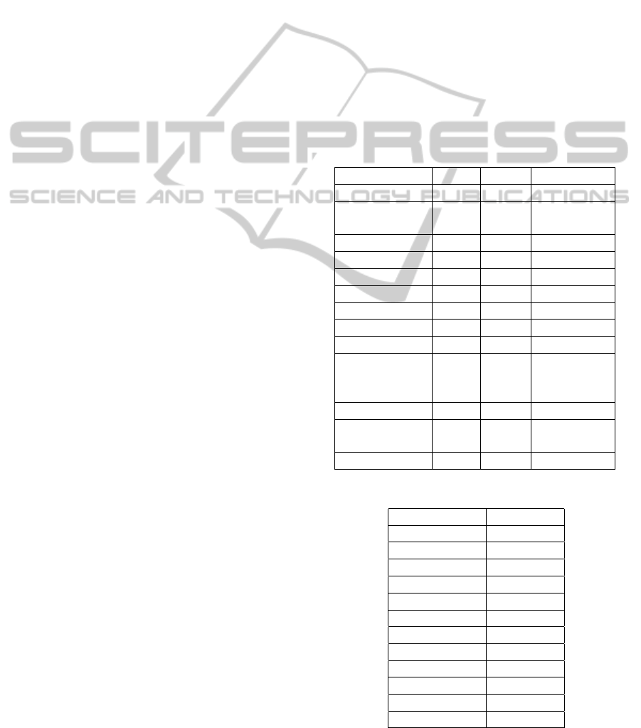
In table 1 each row captures the (possible) differ-

ent SLAs, modeled in term of CPU and memory re-

quirements, for a different kind of virtual machine.

A signiﬁcant share of the total are virtualized desk-

tops, with different ﬂavors for different kind of users

(i.e. a low level desktop would sufﬁce for some cleri-

cal work, whilst an high level desktop is better suited

for some engineering work). Other systems are busi-

ness systems alike as application servers, email sys-

tems and so on. Some of these systems have different

possible SLAs (as an example, a low level desktop

could have 1 CPU and 1 GB of memory or 2 CPU

and 2 GB of memory). We have omitted disk re-

sources, as in a cloud computing environmentthey are

usually centralized on a NAS/SAN system, for which

we have not been able to ﬁnd any sufﬁciently accu-

rate power consumption model. Network resources

are also omitted as they account for a very small part

of the energy consumption. In table 2 there are the

fees that the CSP earns when it allocates one virtual

machine of a speciﬁc kind with a speciﬁc SLA (i.e.,

the CSP earns 0.25 units of currency when it allocates

resources for a low level desktop with 1 CPU and 1

GB of RAM, but earns 0.5 units of currency when al-

locates resources for a low level desktop with 2 CPUs

and 2 GB of RAM). It is important to observe that

these fees are monotone non decreasing in each class

of virtual machines but not necessarily all over the

classes, and any linear relation between fees and the

number of CPUs or memory footprint is generally ap-

plicable but not always true. We have chosen these

fees considering some typical market prices from big

cloud vendors. Table 3 shows some parameters for

a medium blade system, comprised of 2 CPUs of 8

cores each, with each CPU absorbing at full power 90

W. The memory (64 GB) absorbs up to 20 W, and with

an idle power of 100 W the blade at full usage drains

300 W. PUE is set to 1.5 and 1 kWh costs 0.12 units

of currency. In our model we have 32 of these blades

to host virtual machines. As we are considering kWh

as the unit of energy cost, we are implying that the

optimization problem is evaluated on an hourly ba-

sis. On each of these allocation slots we could have a

change of some of the model parameters, as the price

of electricity during off-peak hours is quite lower than

during peak hours. We note that this istance of an NP-

hard problem as an excess of 11,000 decision vari-

ables.

Table 1: Types, numerosity and different SLAs for CPU and

memory requirements for the experimental testbed.

Class Num. CPUs Mem. (GB)

Low Desktop 70 1/2 1/2

Medium

Desktop

50 2/4 2/4

High Desktop 20 4/4 4/8

App Server 8 2/4/6 4/8/8

DB Server 2 2/4/4 4/8/8

Web Proxy 1 4/8 8/16

DSS 1 4 8

Web Server 10 2/4 2/4

File Server 1 1/1 2/4

Knowledge

Management

System

1 2/4 2/4

Intranet 1 1/2 1/2

Software Dis-

tribution

1 2/4 2/8

Email system 4 2/4 2/4

Table 2: Scenario 1: Fees for each class and SLAs.

Low Desktop 0.25/0.5

Med. Desktop 0.50/0.75

High Desktop 1/1.5

App Server 0.50/1.5/2

DB Server 0.5/1.5/1.5

Web Proxy 1.5/2.0

DSS 1.5

Web Server 0.25/0.5

File Server 0.25/0.5

Know. Mgt. 0.5/0.75

Intranet 0.2/0.5

Sw. Dist. 0.5/1.0

Email system 0.5/0.75

SMARTGREENS2012-1stInternationalConferenceonSmartGridsandGreenITSystems

250

Table 3: Parameters for the server. The hourly cost of a

server is the procurement cost amortized over 5 years.

Parameter Value

Physical Host CPUs 16

Physical Host Memory 64 GB

Server Cost 15,000

Server Hourly Cost 0.34

Peak power 300 W

Idle power 100 W

CPU drained power 180 W

Memory drained power 20 W

6 SIMULATION RESULTS

We start observing that the heuristic is heavily depen-

dent on the order of the virtual machines in the prob-

lem, as the basic algorithms producing the initial so-

lutions to improve upon (Next Fit, First Fit, Best Fit)

are such. These algorithms aren’t suited for multiple-

choice knapsack optimization problems, so they ﬁnd

a solution considering only the lowest SLA for each

virtual machine. Also, these algorithms doesn’t offer

any possible tuning, and each one of them produces

just a single solution to the problem. We then perform

a permutation of the virtual machines in the dataset,

because these algorithms are all particularly sensitive

to the ordering (as their names suggest) while chang-

ing it doesn’t produce a new problem but only a pos-

sible different solution. For the heuristic, we have

done 20 random permutations for each initial algo-

rithm, seeing that the resulting differences in the prof-

its are quite narrow. The heuristic is quite fast, with

a computation time of about 2 seconds on a low level

desktop system.

Figure 1 shows the results when the kWh varies

from 0.1 to 1, for PUE=1.5 and C=0.34. If we look

back at table 1, we see that the lowest number of

CPUs to be allocated is 312, requiring a minimum of

341 GBs of RAM. The allocations on ﬁgure 1 results

in 383, 399 or 400 CPUs (the number is dependent

on the permutations of initial data and the speciﬁc

basic algorithm), with respectively 494, 506 or 507

GBs of RAM. The combined resources from the 32

servers are of 512 CPUs and 1024 GBs of RAM. So

the heuristic is better than a simple First/Next/Best Fit

algorithm, as it does ﬁnd some improvements, but at

some point is unable to progress, and it almost ﬁnds a

plateau.

Figure 2 shows the results for different values of

kWh and PUE, for C ﬁxed at 0.34. Clearly, increase

in kWh cost or in PUE results in less proﬁts, and the

surface is almost regular, conﬁrming our analysis on

0.1 0.2 0.3 0.4 0.5 0.6 0.7 0.8 0.9 1

Profit

kWh

Figure 1: Heuristic results with PUE=1.2 and C=0.34.

0.1

0.2

0.3

0.4

0.5

1.2

1.4

1.6

1.8

Profit

kWh

PUE

Profit

Figure 2: Heuristic results with C=0.34.

the limits of this solution technique.

For the GA, we have considered only 600 gen-

erations for each problem instance; a single gener-

ation requires about 3 seconds of computation on a

medium level desktop system, with a code that is not

optimized for speed; as with every genetic algorithm,

these computations are massively parallelizable, so

we don’t consider the time scale as a critical factor.

The GA starts with an initial population (i.e. a set

of solutions) constructed as for the heuristic, i.e. ap-

plying the First Fit, Best Fit and Next Fit algorithms

to the associated bin packing optimization problem

after some random permutations. Then, this popu-

lation is fed to the GA, that starts its optimization

phase. By looking at the population’s average ﬁtness,

we see how the optimization is quite steep at the be-

ginning, then it almost reaches a plateau around 300

generations. The average ﬁtness (which is the sum of

the objective function in eq. 6 and of an evaluation

of the slackness of the proposed allocation) starts at

about 120, then increase linearly as more better solu-

tions are found and enter in the populations removing

worse ones; ﬁnally around 300 generations the local

optimum is found, and so the average ﬁtness of the

population starts to stabilize.

Figure 3 shows the results for different values of

kWh, for a ﬁxed value of PUE set at 1.5. Although

the curve isn’t smooth, it clearly shows a trend: when

the price of kWh increases the proﬁt decreases. This

could be explained both by the effect of the ﬁxed

part of costs (idle power of servers) and by the re-

duced economic convenience in allocating resources

AVIRTUALMACHINESPLACEMENTMODELFORENERGYAWARECLOUDCOMPUTING

251

105

115

0.1 0.4 0.8 1.2 1.6

Profit

kWh

Figure 3: Proﬁts for different values of kWh (PUE=1.5).

for more demanding virtual machines. We see that the

GA outperforms the heuristic almost by a factor of 2.

We lack a way to show the solutions to these dif-

ferent instances in a readable way, but by analytically

looking at them we see that the allocations change

when a model parameter changes. This means, at

ﬁrst, that the GA has successfully been made energy-

aware, incorporating all the energy metrics in the

search for a local optimum (which could or could not

be the global optimum, but either way is a signiﬁcant

improvement over the initial solution). The rough

edges that we see could be explained considering the

general problem is composed of a linear part (energy

costs are almost linear with respect to the amount of

resources) but also of a non-linear part (allocation of

resources does not allow for fractional allocations),

and these two different parts of the model interacts

in an way that appears unintuitive. Also, we have

deﬁned the fees as an almost linear relation of the

resources consumption, and by doing this we have

signiﬁcantly reduced the GA’s ability to leverage on

prices to ﬁnd a more economically convenient alloca-

tion of resources. We don’t see this for the heuristic

because it simply fails to aggressively optimize the

allocations.

7 CONCLUSIONS

We have developed a model that deals with both oper-

ational expenses and capital expenses of a cloud com-

puting system. The Cloud Service Provider has the

economic incentive to maximize its revenues. To do

so, it must take into account all the costs related to the

infrastructure provisioning and day to day operations,

with a major part of them made by electricity costs.

On the other side, the Cloud Service Customer is in-

terested in reducing the fees it has to pay for the cloud

deployment of its infrastructure, but also wants the

biggest ﬂexibility in choosing the right size of its sys-

tems. To successfully manage and compose these two

conﬂicting interests, we have to deploy comprehen-

sive model of resources allocation for a cloud archi-

tecture, where we cannot consider only CPU require-

ments to deﬁne both virtual machines properties, al-

location schema and energy power consumption. The

model should allow for more detailed negotiations be-

tween the two parties, where one or the other could

offer (or ask) for different level of services, also keep-

ing in mind the capacity of the cloud architecture to

accommodate for this and the resulting different op-

erational expenses. The resulting model that we have

developedin this paper offers all of this kind of gener-

ality, and we have developed approximate algorithms

to solve it. Results show that the heuristic fails to ﬁnd

a good solution, while the genetic algorithm performs

better. Also, we consider that a GA is particularly

ﬁtted to this kind of problems, as genetic algorithms

are both easily parallelizable (and cloud computing

has vast and scalable amount of resources) and evolu-

tionary (and cloud computing architectures offers the

ability to change the current allocation of virtual ma-

chines via live migration of them). A ﬁrst analysis

of the model shows that the non-linear part (resources

allocation) interacts in complex ways with the linear

part (energy model), suggesting that more researches

and characterizations of cloud architectures should be

investigated to further analyze this problem which is

of capital importance for the economics of green and

cloud computing.

ACKNOWLEDGEMENTS

We would like to thank Emiliano Casalicchio for his

suggestions and support during the development of

this work. Ancitel SpA generously provided a travel

grant.

REFERENCES

Beloglazov, A. and Buyya, R. (2010). Energy efﬁcient allo-

cation of virtual machines in cloud data centers.

Campegiani, P. (2009). A genetic algorithm to solve the vir-

tual machines resources allocation problem in multi-

tier distributed systems. In 2nd International Work-

shop on Virtualization Performance: Analysis, Char-

acterization and Tools (VPACT'09).

Campegiani, P. and LoPresti, F. (2009). A general model

for virtual machines resources allocation in multi-tier

distributed systems. In 5th International Conference

on Autonomic and Autonomous Systems (ICAS '09).

IARIA.

Cardosa, M., Korupolu, M. R., and Singh, A. (2009).

Shares and utilities based power consolidation in vir-

tualized server environments. In IFIP/IEEE Interna-

SMARTGREENS2012-1stInternationalConferenceonSmartGridsandGreenITSystems

252

tional Symposium in Integrated Network Management

(IM '09). IEEE.

Chang, F., Ren, J., and Viswanathan, R. (2010). Optimal re-

source allocation in clouds. In 3rd IEEE International

Conference on Cloud Computing.

Economou, D., S. Rivoire, C. K., and Ranganatham, P.

(2006). Full-system power analysis and modeling

for server environments. In Workshop on Modeling

Benchmarking and Simulation (MOBS).

Gandhi, A., Harchol-Balter, M., Das, R., and Lefurgy, C.

(2009). Optimal power allocation in server farms. In

SIGMETRICS/Performance '09.

Lu, X. and Gu, Z. (2011). A load-adaptive cloud resource

scheduling algorithm model based on ant colony al-

gorithm. In IEEE Cloud Computing and Intelligent

Systems.

Mazzucco, M. and Dumas, M. (2011). Reserved or on-

demand instances? a revenue maximization model for

cloud providers. In IEEE 4th International Confer-

ence on Cloud Computing.

McCullogh, J., Agarwal, Y., and Chandrashekar, J. (2010).

Evaluating the effectiveness of model-based power

characterization. In USENIX Annual Technical Con-

ference.

Rivoire, S., Ranganathan, P., and Kozyrakis, C. (2008). A

comparison of high-level full-system power models.

In Conference on Power aware computing and sys-

tems (HOTPOWER'08). USENIX.

Singh, K., Bhadauria, M., and McKee, S. A. (2009). Real

time power estimation and thread scheduling via per-

formance counters. ACM SIGARCH Computer Archi-

tecture News, 37(2):46–55.

Srikanthaiah, S., Kansal, A., and Zhao, F. (2008). Energy

aware consolidatin for cloud computing. In Confer-

ence on Power aware computing and systems (HOT-

POWER'08). USENIX.

Urgaonkar, R., Kozat, U. C., Igarashi, K., and Neely, M. J.

(2010). Dynamic resource allocation and power man-

agement in virtualized data centers. In IEEE Network

Operations and Management Symposium (NOMS'10).

AVIRTUALMACHINESPLACEMENTMODELFORENERGYAWARECLOUDCOMPUTING

253

REFERENCES

Beloglazov, A. and Buyya, R. (2010). Energy efficient allo-