PATCHWORK TERRAINS
Luigi Rocca, Daniele Panozzo and Enrico Puppo
DISI, University of Genoa, Via Dodecaneso 35, Genoa, Italy
Keywords:
Terrain Modeling, Multiresolution Modeling, Terrain Rendering.
Abstract:
We present a radically new method for the management, multi-resolution representation and rendering of
large terrain databases. Our method has two main benefits: it provides a C
k
representation of terrain, with k
depending on the type of base patches; and it supports efficient updates of the database as new data come in.
We assume terrain data to come as a collection of regularly sampled overlapping grids, with arbitrary spacing
and orientation. A multi-resolution model is built and updated dynamically off-line from such grids, which
can be queried on-line to obtain a suitable collection of patches to cover a given domain with a given, possibly
view-dependent, level of detail. Patches are combined to obtain a C
k
surface. The whole framework can is
designed to take advantage of the parallel computing power of modern GPUs.
1 INTRODUCTION
Real time rendering of huge terrain datasets is a chal-
lenging task, especially for virtual globes like Google
Earth and Microsoft Virtual Earth, which may need to
manage terabytes of data. Terrains are usually repre-
sented as Digital Elevation Maps (DEMs) consisting
of collections of grids, which may have different res-
olutions and different orientations.
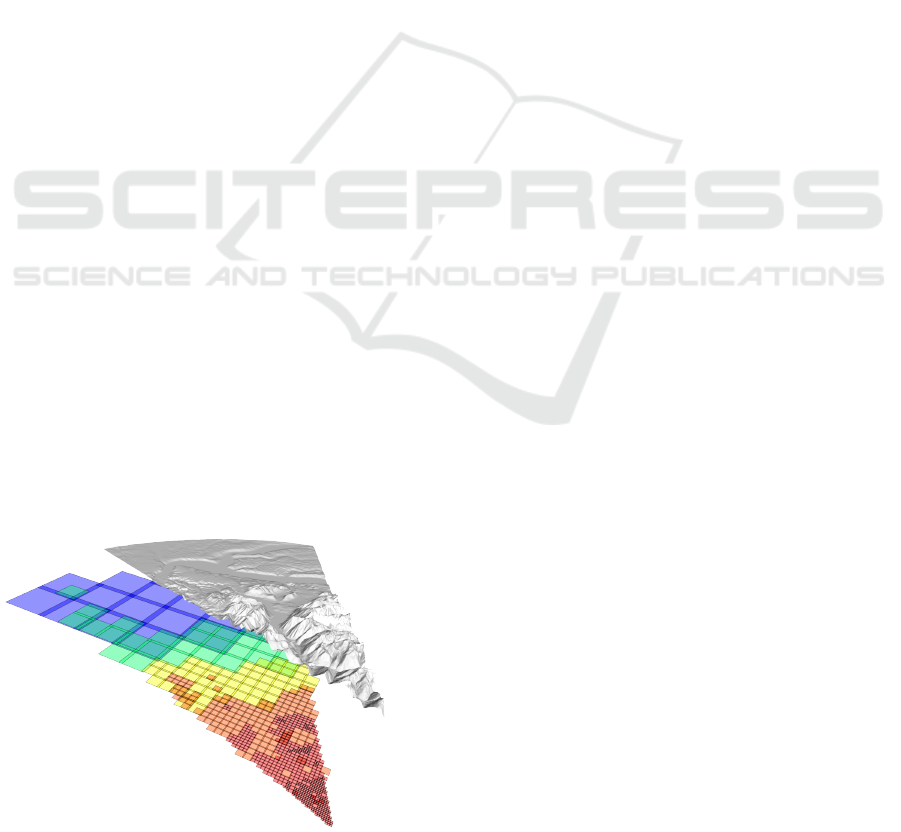
Figure 1: A view-dependent query executed on the Puget
Sound Dataset with an on-screen error of one pixel. The
different colors represent patches of different sizes.
In order to support interactive rendering, manip-
ulation and computation, it is necessary to adopt ap-
proaches that can rapidly fetch a suitable subset of
relevant data for the problem at hand. Such a releva-
nt subset is usually defined in terms of both spatial
domain and resolution. Besides view-dependent ter-
rain rendering, specific GIS applications such as anal-
yses in hydrography, land use, road planning, etc.,
require to handle data at different resolutions.To ef-
ficiently support such tasks, a model featuring Con-
tinuous Level Of Detail (CLOD) is thus necessary.
At the best of our knowledge, all CLOD models in
the literature not only require to pre-process the input
datasets, but also the data structures they use cannot
be updated dynamically with new data (Pajarola and
Gobbetti, 2007).
In this paper, we present an approach to CLOD
terrain modeling that is radically different from previ-
ous literature. Its salient features can be summarized
as follows:
1. Our method produces on-line a compact C
k
rep-
resentation of terrain at the desired accuracy over
a given domain. This representation consists of
a collection of rectangular patches, of different
sizes and orientations, which locally approximate
different zones of terrain at different accuracies.
Patches can freely overlap and they are blended
to obtain a single C
k
function. See Figure 1. The
degree of smoothness k can be selected depending
on application requirements.
2. Starting from the input DEMs, we produce a large
collection of patches of different sizes and accura-
cies, and we store them in a spatial data structure
indexing a three-dimensional space, having two
dimensions for the spatial domain, and a third di-
67
Rocca L., Panozzo D. and Puppo E..
PATCHWORK TERRAINS.
DOI: 10.5220/0003848500670076
In Proceedings of the International Conference on Computer Graphics Theory and Applications (GRAPP-2012), pages 67-76
ISBN: 978-989-8565-02-0
Copyright
c
2012 SCITEPRESS (Science and Technology Publications, Lda.)

mension for the approximation error. Every patch
is represented as an upright box: its basis corre-
sponds to the domain covered by the patch; its
height corresponds to the range of accuracies for
which the patch is relevant. We optimize the range
of accuracies spanned by each patch, so that the
number of patches used to represent a given LOD
is minimized. Independent insertion of patches
in the spatial index can be performed easily and
efficiently, and the result is order independent,
thus dynamic maintenance of the database is sup-
ported.
3. Spatial queries are executed by finding the set
of boxes that intersect a user-defined surface in
the space defined above, depending on the de-
sired LOD. Such a surface may be freely de-
fined according to user’s needs, thus supporting
space culling and CLOD altogether. Incremental
queries are possible, so that efficient transfer of
patches to the GPU is supported: if the result of
a query differs only slightly from the result of the
previous one, it is sufficient to transfer to the GPU
just the new patches that come in, together with
the identifiers of patches to be discarded.
4. The GPU can directly sample this representation
to produce an adaptive (possibly view-dependent)
tessellation with arbitrary connectivity.
This paper describes the general framework,
alongside with two proof-of-concept implementations
of our method. The first implementation is tailored for
real time rendering: it provides a C
0
representation
that can be efficiently sampled in real-time. This rep-
resentation can be evaluated efficiently in parallel and
it is suitable for a GPU implementation. We present
results obtained with our CPU implementation, which
is already able to support real time rendering (25 fps)
on a moderately large dataset (about 256M points)
with an error of one pixel in screen space. The sec-
ond implementation is focused on quality and can be
used for common GIS tasks, such as analyses in hy-
drography, land use, road planning, etc.: it provides a
smooth C
2
representation that can support computa-
tions on terrain using continuous calculus. Both im-
plementations support CLOD queries.
2 RELATED WORK
Overall, known approaches to terrain modeling and
rendering can be subdivided in the four categories re-
viewed in the following. The first category is bet-
ter suited for modeling purposes, while the other
three categories are specifically designed for render-
ing. Our proposal belongs to none of them, and it can
be tailored for both rendering, and other GIS tasks,
with small modifications to a common framework.
CLOD Refinement in CPU. CLOD refinement
methods produce triangle meshes that approximate
the terrain according to LOD parameters that can vary
over the domain (possibly depending on screen or
world space error). They are mostly used for mod-
eling and processing purposes, since they provide an
explicit representation, with the desired trade-off be-
tween accuracy and complexity. Recent surveys on
CLOD refinement methods can be found in (Pajarola
and Gobbetti, 2007; Weiss and De Floriani, 2010).
Cluster Triangulations. Recent GPUs are able to
render many millions of triangles per second, so the
CPU may spend only a few instructions per triangle
in order to prepare data to be rendered in real-time.
This fact has led to the development of methods that
cluster triangles in a preprocessing steps, possibly at
different resolutions, which are then passed to the
GPU and rendered in batches. The rendering prim-
itive is not anymore a single triangle, but rather a tri-
angle strip encoding a large zone of terrain. The chal-
lenge in these approaches is to stitch different clusters
properly. This is usually achieved in a preprocessing
step that guarantees conformality of extracted meshes
(Cignoni et al., 2003). A survey of these approaches
can also be found in (Pajarola and Gobbetti, 2007).
They are usually meant exclusively for rendering pur-
poses.
Geometry Clipmaps. A different approach has
been presented in (Losasso and Hoppe, 2004), where
Geometry Clipmaps are stored in the GPU mem-
ory, and used to render the part of terrain visible
by the user. As the viewpoint moves, the Geometry
Clipmaps are updated in video memory. Tessellation
is performed directly in the GPU. This method takes
advantage of the intrinsic coherence of height maps
to compress the input, thus reducing the amount of
data that are passed to the GPU. With this method,
very high frame rates can be obtained even for huge
datasets.
GPU Ray-casting. The use of ray-casting for ren-
dering height maps is well studied in the literature,
and different GPU techniques that achieve real-time
frame rates have been developed in recent years. In
(Carr et al., 2006), a method to render meshes rep-
resented as Geometry Images is proposed. Follow-
ing a similar approach, specific methods for real-time
GRAPP 2012 - International Conference on Computer Graphics Theory and Applications
68
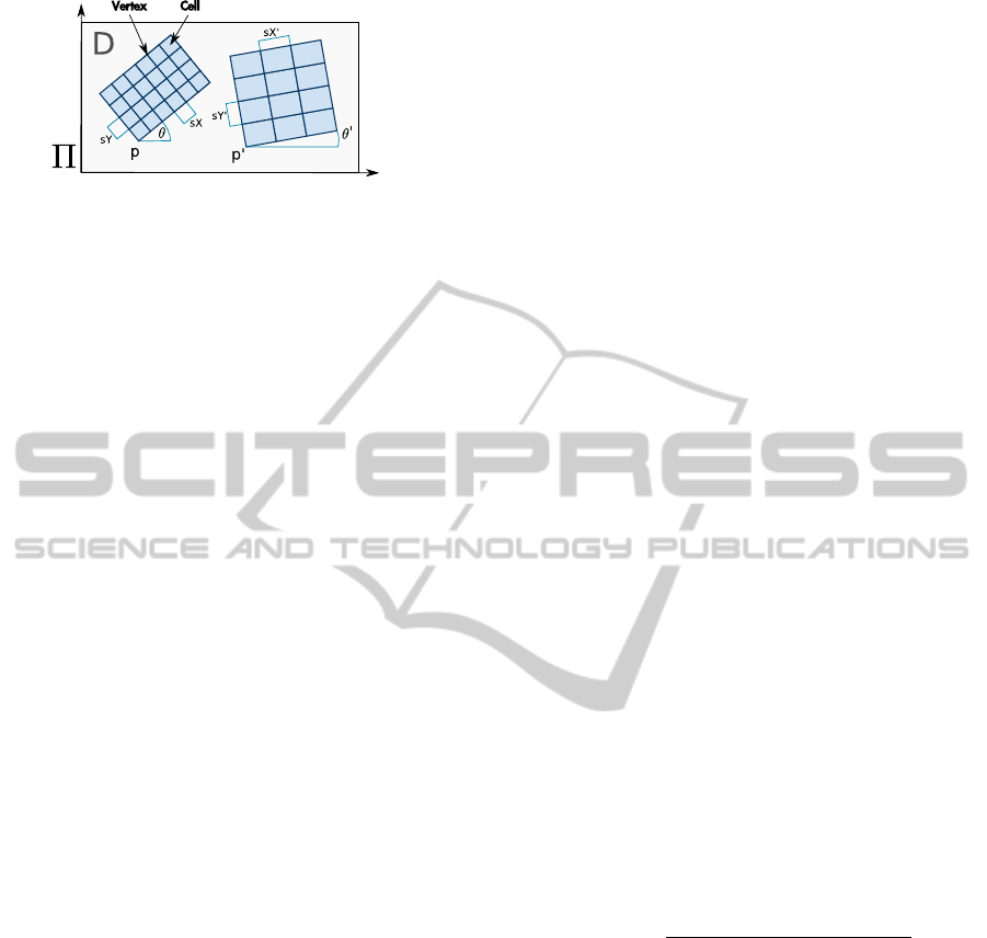
Figure 2: The terrain is covered by a set of regularly sam-
pled grids. Every grid has its own anchor point p, orienta-
tion angle θ and different sample steps for the two axes sX
and sY .
rendering of height maps have been proposed in (Oh
et al., 2006; Tevs et al., 2008). However, all these
methods were not designed to work with large terrain
datasets. In (Dick et al., 2009), a tiling mechanism
is used to support real-time rendering on arbitrarily
large terrains. Ray-casting methods can be used only
for the purpose of rendering, since they do not pro-
duce an explicit multi-resolution representation.
3 PATCHWORK TERRAINS
In this Section, we describe our technique: in Subsec-
tion 3.1, we define the type of patches we use; then, in
Subsection 3.2, we describe how patches are blended
to form a C
k
representation of terrain; finally, in Sub-
section 3.3, we describe the multi-resolution model,
the order-independent algorithm for the dynamic in-
sertion of patches and the spatial queries.
3.1 From Grids to Patches
We assume a two-dimensional global reference sys-
tem Π on which we define the domain D of the terrain,
where all input grids are placed. A grid is a collection
of regularly sampled height values of terrain. In addi-
tion to the matrix of samples, every grid is defined by
an anchor point, an angle that defines its orientation,
and grid steps in both directions (see Figure 2). In
the following, we will use the term vertex to denote a
sample point on the grid, and the term cell to denote a
rectangle in D spanned by a 2×2 grid of adjacent ver-
tices. The accuracy of a grid also comes as a datum,
and it is the maximum error made by using the grid to
evaluate the height of any arbitrary point on terrain.
We aim at defining parametric functions that rep-
resent small subsets of vertices of the grid, called
patches. A single patch is defined by an anchor point,
its height, its width, and the coefficients that describe
the parametric function. For the sake of simplicity,
we will consider the height and width of every patch
to be equal, hence the domain of every patch will be
a square. Extension to rectangular patches is trivial.
We consider two types of patches: perfect patches
interpolate the samples of the original terrain; while
approximating patches only provide an approxima-
tion of the original data. We assign an error to each
patch, namely the accuracy ε of the input grid for a
perfect patch; and ε + δ for an approximating patch,
where δ denotes the maximum distance between a
sample in the input grid and its vertical projection to
the patch. We will denote as kernel a rectangular re-
gion inside every patch, while the rest of the patch
will be denoted as its extension zone.
The type of function defining a patch, as well as
the relation between kernel and extension zones, will
vary depending on the application. In Section 4.1 we
provide specific examples. Our technique, however,
can be used with any kind of parametric function: de-
pending on the application, it may be convenient to
use either a larger collection of simpler patches, or a
smaller collection of more complex patches. The rest
of this section is generic in this respect.
Note that, unlike splines, our patches may freely
overlap, without any fixed regular structure.
3.2 Merging Patches
Given a collection of freely overlapping patches, we
blend them to produce a smooth function that repre-
sents the whole terrain spanned by this collection. In
order to obtain a C
k
surface that is efficient to eval-
uate, we use a tensor product construction, starting
from the one dimensional, compactly supported ra-
dial basis function defined in (Wendland, 1995). Our
weight function is defined as:
W (x, y,d) =
w(x/d)w(y/d))
R
1
−1
R
1
−1
w(x/d)w(y/d) dxdy
for x,y ∈ [−d,d] and 0 elsewhere. The 1-dimensional
weight w(t) is a C
k
function with compact support,
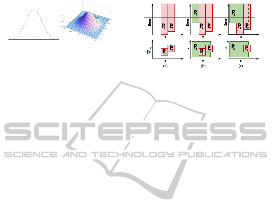
as defined in (Wendland, 1995): see Figure 3 for the
C
2
case and Section 4.1 for further details. It is easy
to see that the weight function W has the following
properties:
1. It has compact support in [−1,1] × [−1, 1];
2. Its derivatives up to order k vanish on the bound-
ary of its support;
3. It is C
k
in [−1,1] × [−1, 1];
4. It has unit volume.
The first three conditions guarantee that the
weight function has limited support, while being C
k
PATCHWORK TERRAINS
69
-1.0
-0.5
0.5
1.0
0.2
0.4
0.6
0.8
1.0
(a) (b)
Figure 3: C
2
weight functions: (a) 1D function w, plot-
ted between -1 and 1. (b) 2D function W , plotted with x,y
between -1 and 1, with the parameter d set to 1.
everywhere. This is extremely important for effi-
ciency reasons, as we will see in the following. Prop-
erty 4 is useful, since it naturally allows smaller (and
more accurate) patches to give a stronger contribution
to the blended surface.
For every patch P, we define its weight function
W
P
(x,y) as a translated and scaled version of W , such
that its support corresponds with the domain of P:
W
P
(x,y) = W (|x − P
x
|,|y − P
y
|,P
s
)
with P
x
and P
y
the coordinates of the center of P and
P
s
the size of P.
A collection of C
k
patches P
1
,P
2
,...,P
n
placed on
a domain D, such that every point of D is contained in
the kernel of at least one patch, defines a C
k
surface
that can be computed using the following formula:
f (x, y) =
∑
n
i=0
P
i
f
(x,y)W
P
i
(x,y)
∑
n
i=0
W
P
i
(x,y)
(1)
with P
i
f
the function associated with patch P
i
.
Note that the surface is C
k
inside D since it is de-
fined at every point as the product of C
k
functions and
the denominator can never vanish since every point in
D belongs to the interior of the domain of at least one
patch. The summation actually runs only over patches
whose support contains point (x,y), since the weight
function will be zero for all other patches.
At this point, terrain can be described with an un-
structured collection of patches. To use this method
on large datasets, we still miss a technique to effi-
ciently compute this representation at a user-defined
LOD.
3.3 The Multi-resolution Model
We build a multi-resolution model containing many
patches at different LODs, and we provide a simple
and efficient algorithm to extract a minimal set of
patches covering a given region of interest at a given
LOD, possibly variable over the domain.
We define a 3D space, called the LOD space, in
which two axes coincide with those of the global ref-
Figure 4: Boxes of patches in LOD space, with a cut shown
by the blue line: (a) Two independent patches P
1
and P
2
; (b)
A third patch P
3
is added: patch P
1
becomes redundant for
the given cut; (c) P
1
is shortened to obtain a minimal set of
patches for every cut of the spatial index.
erence system Π, while the third axis is related to ap-
proximation error. For simplicity, we will set a maxi-
mum allowed error, so that LOD space is bounded in
the error dimension. In this space, every patch will be
represented as an upright box (i.e., a parallelepiped),
having its basis corresponding to the spatial domain
of the patch, and its height corresponding to the range
of approximation errors, for which the patch is rel-
evant. The bottom of the box will be placed at the
approximation error of the patch, while its top will be
set to a larger error, depending on its interaction with
overlapping boxes, as explained in the following.
In this section, patches will be always treated as
boxes, disregarding their associated functions. We
will consider open boxes, so that two boxes sharing
a face are not intersecting. For a box B, we will de-
note as B.min and B.max its corners with minimal and
maximal coordinates, respectively. Furthermore for a
point p in LOD space, we will denote its three coor-
dinates as p.x, p.y and p.z.
Given a collection of patches embedded in LOD
space, a view of terrain at a constant error e can be
extracted by gathering all boxes that intersect the hor-
izontal plane z = e. More complex queries, which
may concern a region of interest as well as variable
LOD, can be obtained by cutting the LOD space with
trimmed surfaces instead of planes.
To informally describe our approach, let us con-
sider the examples depicted in Figure 4. Figure
4(a) shows two non-overlapping patches embedded
in LOD space: P
1
is a perfect patch with zero er-
ror, and its box extends from zero to maximum error
in the LOD space. This means that P
1
will be used
to approximate its corresponding part of terrain at all
LODs. On the contrary, patch P
2
is an approximating
patch: it has its bottom set at its approximation error,
while its top is again set at maximum error. Patch P
2
will be used to represent its part of terrain at any er-
ror larger or equal than its bottom, while it will not be
GRAPP 2012 - International Conference on Computer Graphics Theory and Applications
70

used at finer LODs.
In Figure 4(b), a larger patch P
3
is added to our
collection, which has a larger error than P
1
and P
2
and
also it completely covers P
1
. A cut at an error larger
than the error of P
3
would extract all three patches,
but P
1
is in fact redundant, since its portion of terrain
is already represented with sufficient accuracy from
P
3
, which also covers a larger domain. In order to
obtain a minimal set of patches, in Figure 4(c) patch
P
1
is shortened in LOD space, so that its top touches
the bottom of P
3
. Note that we cannot shorten P
2
in a
similar way, because a portion of its spatial domain is
not covered by any other patch.
This simple example leads to a more complete
invariant that patches in LOD space must satisfy to
guarantee that minimal sets are extracted by cuts. We
first formally describe this invariant, then we provide
an algorithm that allows us to fill the LOD space in-
crementally, while satisfying it. This algorithm builds
the multi-resolution model and the result is indepen-
dent of the order of insertion of patches. Implementa-
tion will be described later in Section 4.2.
We define a global order < on patches as follows:
P < P
0
if the area of P is smaller than the area of P
0
;
if the two areas are equal, then P < P
0
if P.min.z >
P
0
.min.z, i.e., P is less accurate than P
0
.
Since both the spatial extension and the approxi-
mation error of a patch P are fixed, the spatial invari-
ant is only concerned with the top of P, i.e., with its
maximal extension in the error dimension.
Patch Invariant. A patch P must not intersect any
set of patches, such that the union of their kernels
completely covers the kernel of P, and each patch is
greater than P in the global order <. Also, the patch
P cannot be extended further from above without vi-
olating the previous condition.
In other words, this invariant states that a patch is
always necessary to represent terrain at any LOD, in
its whole extension in the error domain, because that
portion of terrain cannot be covered by larger patches.
If all the patches in the model satisfy this property, we
are sure that we will obtain a minimal set of patches
whenever we cut the model with horizontal planes of
the form z = c. The second part of the invariant forces
patches to span all levels of error where their contribu-
tion is useful for terrain representation, thus maximiz-
ing the expressive power of the model. More general
cuts will also extract correct representations in terms
of LOD, but minimality is not guaranteed.
Let us consider inserting a new patch P into a col-
lection of patches that satisfy the invariant. If the new
patch does not satisfy the invariant, we shorten it at its
top. This is done through Algorithm 1 described be-
low. Note that a patch may be completely wiped out
by the shortening process: this just means that it was
redundant. After the insertion of P, only patches that
intersect P may have their invariance property invali-
dated, so we fetch each of them and we either shorten
or remove it, again by Algorithm 1. All this process
is done through Algorithm 2. Shortening patches that
were already in the model does not invalidate invari-
ance of other patches, so no recursion is necessary.
Algorithm 1: cutter(Patch P, SetOfPatches ps).
1: sort ps in ascending order wrt min.z
2: current = {}
3: last = {}
4: for P
0
∈ ps do
5: if P ¡ P’ then
6: current = current ∪ {P
0
}
7: if the patches in current cover P then
8: last = P
0
9: break
10: end if
11: end if
12: end for
13: if not (last == {}) then
14: if last.min.z ¡ P.min.z then
15: Remove P
16: else
17: P.max.z = P
0
.min.z
18: end if
19: end if
Algorithm 2: add-patch (Patch P).
1: ps = patches that intersect P
2: cutter(P, ps)
3: for P
0
∈ ps do
4: if P
0
still intersects P then
5: ps
0
= patches that intersect P
0
6: cutter(P
0
, ps
0
)
7: end if
8: end for
It is easy to see that all patches in a model built
by inserting one patch at a time through Algorithm 2
satisfy the invariant. We also show that the result is
independent on the order patches were added.
Order Independence. The structure of a model built
by repeated application of Algorithm 2 is independent
of the insertion order of patches.
Proof. The height of the box associated to a patch de-
pends only on the spatial position and minimal error
of the other patches inserted in the spatial index. The
invariant guarantees that all boxes have their maxi-
mum allowed size in the error dimension, with respect
PATCHWORK TERRAINS
71

to all other patches in the model. Therefore, the fi-
nal result only depends on what patches belong to the
model.
To summarize, the algorithm shown allows us to
build a spatial data structure that automatically detects
redundant data. Queries are executed by cutting such
structure with planes or surfaces. Extracted patches
are merged, as explained in Section 3.2, to produce
the final terrain representation.
This completes the theoretical foundations of our
technique. We discuss the implementation details in
Section 4, while we provide benchmarks and results
in Section 6.
4 IMPLEMENTATION
This section describes a possible implementation of
the general framework presented in Section 3, which
has been kept as simple as possible for the sake of
presentation. In Section 4.1 we describe the construc-
tion of patches, while in Section 4.2 we describe the
implementation of the spatial index.
4.1 Generation of Patches
We describe two types of patches: bilinear patches
provides a C
0
representation of the terrain that can
be used for rendering purposes; while bicubic patches
provide a C
2
representation, trading speed for in-
creased terrain quality.
We use patches at different scales, which are
generated from sub-grids of the various levels of a
mipmap of terrain data. Each patch is a rectangle that
covers a set of samples of the terrains. The patch must
represent the terrain it covers, and its size depends on
the density of grid samples. Patches may also cover
mipmaps, thus allowing to represent larger zones of
the terrain with less samples.
For every level of the mipmap, we build a grid of
patches such that the union of their kernels form a
grid on the domain, and the intersection of their ker-
nel is empty. The size of the kernel with respect to the
size of the patch is a parameter controlled by the user,
that we denote σ. Any value 0 < σ < 1 produces a
C
k
terrain representation; different values can be used
to trade-off between quality and performance: small
values of σ improve the quality of blending between
patches; conversely, large values reduce the overlap-
ping between different patches, thus improving effi-
ciency, but transition between different patches may
become more abrupt, thus producing artifacts. In our
experiments, we use σ = 0.9.
Bilinear Patches. are formed by a grid of samples
and they are simply produced by bilinear interpola-
tion of values inside every 2x2 sub-grid of samples.
These patches are C
0
in their domain, and the blend-
ing function we use is obtained by w(t) = (1 − |t|).
Bicubic Patches. are formed by a grid of samples,
as in the case of bilinear patches. To define a piece-
wise bicubic interpolating function we compute an in-
terpolant bicubic spline with the algorithm described
in (Press et al., 2007). These patches are C
2
in their
domain, and the blending function we use is w(t) =
(1 − |t|)
3
(3|t| + 1).
4.2 Spatial Index
The spatial index must support the efficient insertion
and deletion of boxes, as well as spatial queries, as ex-
plained in Section 5.1. An octree would be an obvious
choice, but it turns out to be inefficient, because large
patches are duplicated in many leaves. We propose
here a different data structure that is more efficient
for our particular application.
We build a quadtree over the first two dimensions,
storing in every node n (either internal or leaf) the set
of patches that intersect the domain of n. Not all inter-
secting patches are stored, but just the first t patches
that have their highest value on the z-axis, and that are
not stored in any ancestor node of n. We use a thresh-
old t of 64 in our experiments. There is no guarantee
that a patch is stored in exactly one node, but in our
experiments a patch is always stored in less than two
nodes on average.
This data structure can be seen as a set of lists of
patches, ordered depending on their highest value on
the z-axis. Such a set is subsequently split into sub-
lists depending on the spatial domain of patches, in
a way similar to Multiple Storage Quadtrees (Samet,
2005). A visit of the tree produces an ordered list of
the patches that depends only on the spatial domain of
the query surface. This list can then be efficiently an-
alyzed to retrieve the patches that intersect the query
surface, since it is ordered on a key defined on the
third dimension.
Inserting a new box in the tree is simple. Starting
at the root, a box B is inserted in the node(s) that inter-
sects its spatial domain, if and only if either the num-
ber of patches in such node does not exceed its capac-
ity, or the highest z-value of the new box is larger than
the highest z-value of at least another box in the list at
that node; in the latter case, the box in the list with the
minimum highest z-value is moved downwards in the
tree. Otherwise, the new patch is moved downwards
in the tree.
GRAPP 2012 - International Conference on Computer Graphics Theory and Applications
72

As explained in Section 3.3, queries are specified
by a surface in LOD space. The projection of such a
surface in the spatial domain is the region of interest
(ROI) of the query. The z-values of the surface define
the error tolerance at each point in the ROI. At query
time, the quadtree is traversed top-down, and quad-
rants that intersect the ROI are visited. For each such
quadrant, only boxes that intersect the query surface
are extracted. When a node n is visited, the query is
propagated to lower levels only if the lowest z-value
of the query surfaces inside the domain covered by n
is less than the highest z-value of all boxes in n.
5 EXTENSIONS FOR REAL TIME
TERRAIN RENDERING
In this Section, we discuss in detail how view-
dependent queries can be executed in our framework
(Section 5.1) and how our terrain representation is
sampled to produce the triangle strip representation
used for rendering (Section 5.2).
5.1 View-dependent Queries
A view-dependent query is needed to minimize the
computational effort required to correctly represent
the terrain region of interest. For example, during ren-
dering it is possible to represent with lower resolution
areas that are far from viewer, without introducing vi-
sual artifacts.
In Section 3.3, a uniform query is executed by cut-
ting the LOD space with a plane parallel to the spatial
domain. A view-dependent query is more complex
since it involves cutting the spatial index with a more
complex surface.
In (Lindstrom et al., 1996) a method was proposed
that computes the maximum error in world coordi-
nates that we can tolerate, in order to obtain an error
in screen coordinates smaller than one pixel. Such a
method defines a surface in LOD space that we could
use to make view-dependent queries in our spatial in-
dex. However, the resulting surface is complex and
the related intersection tests would be expensive. We
use an approximation of such a method that allows us
to cut the spatial index with a plane, which provides
a conservative estimate of the correct cutting surface:
we obtain a surface that is correct in terms of screen
error, while it could be sub-optimal in terms of con-
ciseness).To compute the cutting plane, we ignore the
elevation of the viewer with respect to the position of
the point, obtaining the the following formula:
δ
screen
=
dλδ
p
(e
x
− v
x
)
2
+ (e
y
− v
y
)
2
,
with e being the viewpoint, v the point of the terrain
where we want to compute the error, d the distance
from e to the projection plane, λ the number of pixels
per world coordinate units in the screen xy coordinate
system, δ the error on world coordinate and δ
screen
the
error in pixel.
This plane is reduced to a triangle by clipping
the zones outside the view frustum. The spatial in-
dex is then cut with this triangle, and the intersection
between boxes in the index and the triangle are ef-
ficiently computed with the algorithm of (Voorhies,
1992), after an appropriate change of reference sys-
tem has been performed on the box.
5.2 Terrain Tessellation
So far, we have shown how to extract a parametric C
k
representation of terrain at the desired LOD. To ren-
der the terrain, we rasterize it by imposing a position-
dependent grid on the domain and by evaluating the
parametric surface only at the vertices of such grid.
We produce a grid that has approximately the same
number of samples as the number of pixels on the
screen, and we define the grid in polar coordinates,
thus obtaining a mesh with a high density of vertices
in the neighborhood of the viewer and with progres-
sively lower densities as we move farther. For the sake
of brevity, we skip the details on the construction of
this grid and we focus on the efficient evaluation of
the view-dependent terrain representation at its ver-
tices.
Let G be a grid on the domain of terrain and let
S be a set of patches extracted from the spatial in-
dex with a view-dependent query. Equation (1) can
be evaluated efficiently by observing that the weight
function associated with a patch P is zero for all the
vertices of the grid that lies outside the domain of P.
Thus, for every patch P
i
, we need to evaluate P
i
f
and
W
P
i
just for the vertices of G that lie in the domain of
P
i
.
We have built a two-dimensional spatial index on
the domain on the terrain that contains the position of
all vertices of G and that allows us to rapidly fetch all
vertices contained in the domain of a patch. We use
a uniformly spaced grid in our prototype. Note that
this spatial index has to be built just once, since the
grid depends only on the position of the viewer. At
each frame, we do not move the grid, but we rather
translate and rotate the patches returned by the query
to place the grid in the desired position. By using
this spatial index, we can efficiently extract the ver-
tices that lie in every patch and incrementally com-
pute Equation (1).
Since the terrain is represented by a parametric
PATCHWORK TERRAINS
73

function, it may be also possible to render it efficiently
with ray-tracing. We plan to investigate this opportu-
nity as well as other ways to triangulate the parametric
representation of the terrain in our future work.
6 RESULTS
In this Section we present the results obtained with
our prototype implementation on a dataset over the
Puget Sound area in Washington. Experiments were
run on a PC with a 2.67Ghz Core i5 processor
equipped with 4Gb of memory, using a single core.
The dataset is made up of 16,385 × 16,385 vertices at
10 meter horizontal and 0.1 meter vertical resolution
(USGS and The University of Washington, 2011).
Our prototype performs all computation on a single
CPU core and achieves interactive rendering frame
rates. In a flight over the Puget Sound datasets, our
framework obtains an average of 25 fps, producing
320k triangles per frame with an on-screen error of 1
pixel.
As we will show, the majority of time is spent
in the rasterization of terrain, which could be paral-
lelized easily on the GPU. If we disable the rasteri-
zation, our system is able to respond to hundreds of
queries per second. We expect that a GPU implemen-
tation, which will be the focus of our future work, will
be able to obtain interactive frame rates on large ter-
rains with HD quality, while using only a subset of
the cores available on modern GPUs.
Sections 6.1, 6.2, 6.3 and 6.4 present results pro-
duced using bilinear patches. Section 6.5 discusses
the performance when bicubic patches are used.
6.1 Pre-processing time
The preprocessing computations executed by our sys-
tem can be divided in three phases: mipmap genera-
tion, error evaluation and construction of the spatial
index. Table 1 reports our preprocessing times for the
full dataset, and for two scaled versions. Note that
pre-processing is performed online, i.e. it is possible
to add new data to a precomputed dataset without the
need to rebuild it from scratch. This feature is unique
of our method since, at the best of our knowledge, it
is not available in any other work in the literature (Pa-
jarola and Gobbetti, 2007).
In our experiments, each patch covers a grid of
32x32 samples, while its kernel is made of the central
28x28 pixels.
The majority of time is spent on the first two
phases, which would be simple to execute in parallel
on multiple cores, unlike the last phase that involves
complex data structures.
6.2 Space Overhead
On average, our multi-resolution model requires
approximately 35% space more than the original
dataset. A breakdown of the space occupied by the
various components of our model is shown in Table
1. The majority of space is taken by the mipmap.
There is a tradeoff between the space occupied by
the multi-resolution model and the size of patches.
Smaller patches increase adaptivity but take more
space since they must be inserted and stored in the
spatial index.
6.3 Uniform Queries
Our system is able to execute 800 uniform queries
per second with a 50m error. Queries with no error
slow down the system to 55 queries per second. Note
that the latter queries return the maximum number of
patches at the highest level of detail possible.
, yielding the highest number of patches an the
most detailed representation possibile, can be exe-
cuted 55 times in a second. Figure 5 shows the re-
sults of three different queries performed with an er-
ror threshold of 5, 20 and 50 meters. Smaller patches
are used to correctly represent fine details, while large
patches are used in flat zones, even with a very low er-
ror threshold. High frequency detail is obviously lost
as error increases.
6.4 View-dependent Queries
A single view-dependent query representing a portion
of terrain 15km long with an on-screen error of one
pixel extracts approximately 250 patches and requires
only 2.5ms. Thus, our system is able to query the
spatial index at very high frame rates, meaning that
the CPU time required for every frame is negligible.
In our prototype, about 95% of the time is spent in
evaluating terrain elevations using Equation 1. This
task is intrinsically parallel, since it can be performed
separately for every vertex of the grid, so we expect
to easily obtain impressive frame rates by demand-
ing to the GPU the evaluation procedure. Figure 6
also shows the number of view-dependent queries per
second executed by our prototype and the number of
extracted patches at different screen error thresholds.
The use of progressive spatial queries could further
increase performance.
In a GPU implementation of our technique, the
query will be executed by the CPU, while the GPU
GRAPP 2012 - International Conference on Computer Graphics Theory and Applications
74
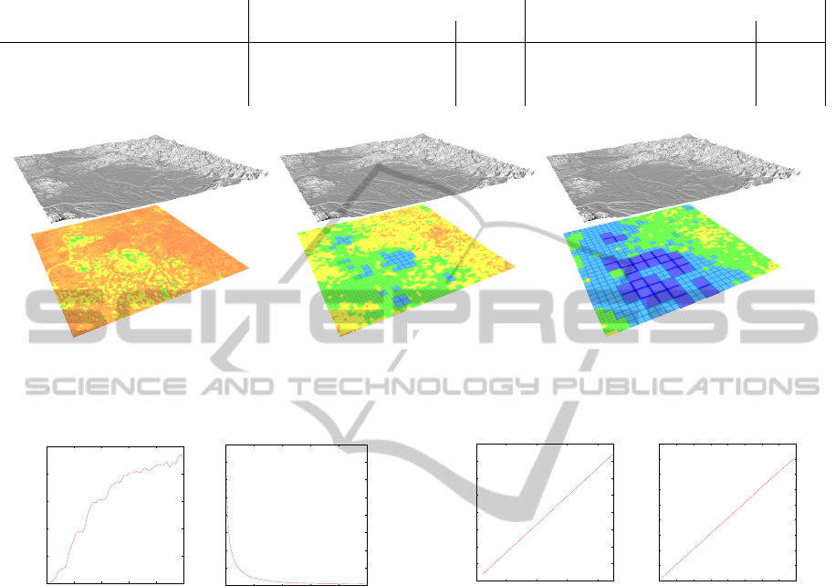
Table 1: Time and space required to preprocess and store the multi-resolution model. From left to right: the time required
to compute the mipmap, to evaluate the error associated with each patch and to build the spatial index; the space required to
store the mipmaps, the patches and the spatial index.
Preprocessing Time Space overhead
Dataset samples Dataset size Mipmap Error Index Total Mipmaps Patches Index Total
1k × 1k 2M 0.1s 0.6s 0.05s 0.75s 702k 18k 12k 732k
4k × 4k 32M 0.9s 10s 0.83s 11.73s 11.2M 301k 202k 11.7M
16k × 16k 512M 12.6s 169s 14.6s 196.2s 179M 4.8M 3.2M 187M
Figure 5: Puget Sound Dataset (16k x 16k samples) rendered with error thresholds of 5, 20 and 50 meters. The colors on the
bottom represent the size of the patch used to approximate the terrain. Blue and cyan corresponds to large patches, used to
approximate flat zones, while red and orange indicates small patches required to represent fine details.
500
1000
1500
2000
2500
3000
0 1 2 3 4 5
Queries per Second
Error (pixels)
(a)
0
500
1000
1500
2000
2500
3000
3500
4000
0 1 2 3 4 5
Extracted Patches
Error (pixels)
(b)
Figure 6: Number of queries per second (a) and number
of extracted patches (b) while performing view-dependent
queries at different screen error thresholds.
evaluates Equation 1 and rasterizes the resulting ter-
rain. Between different frames, only the difference
between the two queries must be sent to the GPU.
We have simulated the traffic between CPU and GPU,
during a fly over the dataset at different speeds: only a
few kb per frame were required to send the difference
between two queries to the GPU (see Figure 7). Every
patch that has to be sent to the GPU uses 4106 bytes,
while the removal of a patch requires only to transfer
its unique identifier (4 bytes).
6.5 Differences with Bicubic Patches
Changing type of patches influences differently the
various steps of our framework. The preprocessing
step is slowed down thirty times: this is due to the
0
200
400
600
800
1000
1200
1400
1600
40 80 120 160
Bandwidth Usage (bytes/frame)
Speed (m/s)
(a)
2000
4000
6000
8000
10000
12000
14000
16000
18000
20000
0.1 0.2 0.3 0.4 0.5 0.6 0.7 0.8 0.9
Bandwidth Usage (bytes/frame)
Speed (rad/s)
(b)
Figure 7: During a straight fly over terrain at different
speeds, only a few bytes per frame must be sent to the
GPU (a). A rotation of the viewpoint requires slightly more
bandwidth (b). Both tests were performed with an allowed
screen error of three pixels and every query extracted 70
patches on average, representing a portion of terrain 15km
long.
huge increase of the computational cost required for
the evaluation of the bicubic patches. The construc-
tion of the spatial index is almost unaffected by the
modification, since the only information that it needs
is the maximal error associated with every patch. The
space used is similar. The evaluation of the terrain is
greatly slowed down and we could obtain just one fps
with the CPU implementation. While our current im-
plementation can be used just for modeling purposes,
a GPU implementation is required to achieve interac-
tive rendering frame rates with bicubic patches.
PATCHWORK TERRAINS
75

7 CONCLUDING REMARKS
We have presented a novel technique for represent-
ing and manipulating large terrain datasets. Its main
advantage is the possibility to efficiently update the
system with new heterogeneous grids, a character-
istic that is not found in any existing method. The
system automatically detects and removes redundant
data. Furthermore, our technique produces a multi-
resolution C
k
surface instead of a discrete model. The
actual evaluation of the surface, which is the only
computationally intensive task, can be demanded to
the GPU, while keeping the communication between
CPU and GPU limited. Texture and normal map can
be easily integrated, since they can be associated to
every patch and interpolated, with the same method
used for the height values.
The space overhead required by the multi-
resolution model is approximately the same as the
space used for a mipmap pyramid, thus it is suitable
to be used even with huge terrains. A limitation of
this technique is the lack of a theoretical bound on the
maximum number of patches that may overlap at a
single point of terrain. This can probably be avoided
if we insert additional criteria to the patch invariant
we use for building the spatial index, and it will be
one of the main points of our future work. However,
in our experiments the number of overlapping patches
never exceeded six, and it was four on average.
We have presented results obtained with our CPU
implementation, which is already able to obtain in-
teractive rendering frame rates using a single core on
moderately large terrains. The algorithm for the con-
struction and update of the multi-resolution model, as
well as the query algorithms are efficient and capable
to manage huge datasets.
We are currently working on a GPU implemen-
tation and the most relevant aspects to achieve effi-
ciency are: incremental queries, providing a stream
of differences between patches defining terrain in the
previous and current frame, which can be directly
transferred to the GPU; efficient update of the list of
patches maintained in the GPU; and the strategy for
parallel evaluation and meshing of terrain.
REFERENCES
Carr, N. A., Hoberock, J., Crane, K., and Hart, J. C. (2006).
Fast gpu ray tracing of dynamic meshes using ge-
ometry images. In Gutwin, C. and Mann, S., ed-
itors, Graphics Interface, pages 203–209. Canadian
Human-Computer Communications Society.
Cignoni, P., Ganovelli, F., Gobbetti, E., Marton, F., Pon-
chio, F., and Scopigno, R. (2003). Bdam - batched dy-
namic adaptive meshes for high performance terrain
visualization. Comput. Graph. Forum, 22(3):505–
514.
Dick, C., Kr
¨
uger, J., and Westermann, R. (2009). GPU ray-
casting for scalable terrain rendering. In Proceedings
of Eurographics 2009 - Areas Papers, pages 43–50.
Lindstrom, P., Koller, D., Ribarsky, W., Hodges, L. F.,
Faust, N., and Turner, G. A. (1996). Real-time, con-
tinuous level of detail rendering of height fields. In
SIGGRAPH ’96: Proceedings of the 23rd annual con-
ference on Computer graphics and interactive tech-
niques, pages 109–118, New York, NY, USA. ACM.
Losasso, F. and Hoppe, H. (2004). Geometry clipmaps:
terrain rendering using nested regular grids. In SIG-
GRAPH ’04: ACM SIGGRAPH 2004 Papers, pages
769–776, New York, NY, USA. ACM.
Oh, K., Ki, H., and Lee, C.-H. (2006). Pyramidal displace-
ment mapping: a gpu based artifacts-free ray tracing
through an image pyramid. In Slater, M., Kitamura,
Y., Tal, A., Amditis, A., and Chrysanthou, Y., editors,
VRST, pages 75–82. ACM.
Pajarola, R. and Gobbetti, E. (2007). Survey of semi-regular
multiresolution models for interactive terrain render-
ing. Vis. Comput., 23(8):583–605.
Press, W. H., Teukolsky, S. A., Vetterling, W. T., and Flan-
nery, B. P. (2007). Numerical Recipes 3rd Edition:
The Art of Scientific Computing. Cambridge Univer-
sity Press, 3 edition.
Samet, H. (2005). Foundations of Multidimensional and
Metric Data Structures (The Morgan Kaufmann Se-
ries in Computer Graphics and Geometric Model-
ing). Morgan Kaufmann Publishers Inc., San Fran-
cisco, CA, USA.
Tevs, A., Ihrke, I., and Seidel, H.-P. (2008). Maximum
mipmaps for fast, accurate, and scalable dynamic
height field rendering. In Haines, E. and McGuire,
M., editors, SI3D, pages 183–190. ACM.
USGS and The University of Washing-
ton (2011). Puget sound terrain.
http://www.cc.gatech.edu/projects/large
models/ps.html.
Voorhies, D. (1992). Triangle-cube intersection. Graphics
Gems III, pages 236–239.
Weiss, K. and De Floriani, L. (2010). Simplex and diamond
hierarchies: Models and applications. In Hauser, H.
and Reinhard, E., editors, Eurographics 2010 - State
of the Art Reports, Norrk
¨
oping, Sweden. Eurographics
Association.
Wendland, H. (1995). Piecewise polynomial, positive defi-
nite and compactly supported radial functions of mini-
mal degree. Advances in Computational Mathematics,
4(1):389–396.
GRAPP 2012 - International Conference on Computer Graphics Theory and Applications
76
