SEGMENTATION OF PLANAR STRUCTURES IN BIOIMAGING

A. Martinez-Sanchez

, I. Garcia

and J. J. Fernandez

Grupo Supercomputacion y Algoritmos, Universidad de Almeria, Almeria, Spain

Grupo Supercomputacion y Algoritmos, Universidad de Malaga, Malaga, Spain

Centro Nacional de Biotecnologia (CSIC), Madrid, Spain

Keywords:

Planar Structures, Segmentation, Feature Detection, Biomedical Imaging.

Abstract:

This work presents an approach to detection of planar structures in three-dimensional (3D) datasets obtained

by different bioimaging modalities. The strategy has already turned out to be effective to segment membranes

from 3D volumes in the ﬁeld of electron tomography, an emerging and powerful technique in structural and

cellular biology. This approach can also be useful to detect planar structures in general in other bioimaging

modalities. The goal of this position paper is to present this approach to the computer vision community and

illustrate the performance on a number of representative bioimaging datasets.

1 INTRODUCTION

The advent of biological imaging has made it possi-

ble to observe, directly or indirectly, the molecular

and cellular architecture and interactions that under-

lie essential functions within cells and tissues (Chan-

dler and Roberson, 2009). The availability of imaging

techniques (optical, confocal, electron microscopies,

electron tomography, just to name a few) in biology

laboratories is growing rapidly. So does the need

for image processing methods that facilitate analy-

sis and interpretation at different scales of resolution

and complexity. In this regard segmentation, which

intends to semantically decompose the datasets into

their structural components, plays a central role.

Structures that can be considered as planes at lo-

cal scale are often found in bioimaging datasets. Bi-

ological membranes are one of the best examples.

Membranes encompass compartments within biolog-

ical specimens, deﬁne the limits of the intracellular

organelles and the cells themselves, etc. Detection

of planar structures in general is important towards

(semi-)automated segmentation of the whole datasets.

Recently, we have presented an approach based on

local differential information that succeeds in seg-

menting biological membranes (or any planar struc-

ture in general) in three-dimensional (3D) datasets

obtained by electron tomography (ET) (Martinez-

Sanchez et al., 2011). ET nowadays proves to be one

of the leading techniques for visualizing the molecu-

lar organization of the cell environment (Frank, 2006;

Lucic et al., 2005). In this ﬁeld, manual segmentation

still remains prevalent because no computational me-

thod has stood out as general applicable yet due to dif-

ferent reasons (they were case-speciﬁc, or limited per-

formance under low signal-to-noise ratio, difﬁcult pa-

rameter tuning, user-intervention required, etc) (Volk-

mann, 2010). In manual segmentation, the user delin-

eates the features of interest using visualization tools,

which is tedious and subjective.

This position paper aims to present our approach

to detect planar structures to the computer vision

community and show its performance on datasets de-

rived from different bioimaging modalities, includ-

ing others than ET. Based on a Gaussian model for

the thickness of the planes, the procedure relies on

the characterization of structures at a local scale us-

ing differential information. Later, the integration at a

global scale yields the deﬁnite detection.

2 DETECTION OF PLANES

2.1 Model for the Planar Structure

In experimental datasets and at a local level, the pla-

nar structure has certain thickness and the density

along the direction normal to the plane progressively

decreases as a function of the distance to the centre of

the plane (Fig. 1) (Fernandez and Li, 2003; Fernandez

and Li, 2005). This density variation can be modelled

by a Gaussian function (Fig. 1):

I(r) =

√

2πσ

−

2σ

(1)

Martinez-Sanchez A., Garcia I. and J. Fernandez J..

SEGMENTATION OF PLANAR STRUCTURES IN BIOIMAGING.

DOI: 10.5220/0003819800420047

In Proceedings of the International Conference on Computer Vision Theory and Applications (VISAPP-2012), pages 42-47

ISBN: 978-989-8565-04-4

 2012 SCITEPRESS (Science and Technology Publications, Lda.)

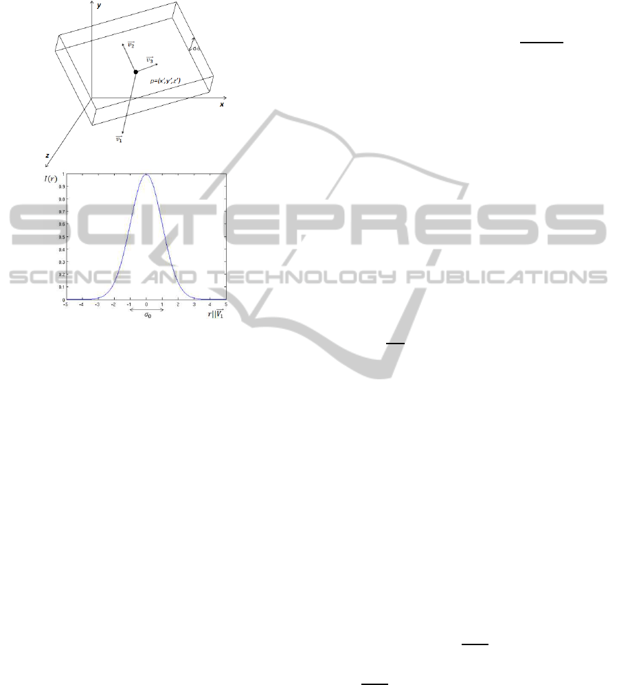
where r runs along the normal to the plane, D

is a

constant to set the maximum density value (at the cen-

tre of the plane) and σ

is related to its thickness.

Figure 1: Plane model and the density proﬁle across it.

The eigen-analysis of the density function at

point p = (x,y,z) of the plane yields the eigenvec-

tors

−→

and

−→

with eigenvalues |λ

| >> |λ

| ≈

|λ

| (Fig. 1) (Fernandez and Li, 2003; Fernandez and

Li, 2005). This reﬂects that there are two directions

(

−→

) with small density variation and the largest

variation runs along the direction perpendicular to the

plane (

−→

, parallel to r, i.e.

−→

||r ).

2.2 Scale-space

The scale-space theory was formulated in the

80s (Koenderink, 1984; Witkin, 1983) and allows

isolation of the information according to the spatial

scale. At a given scale σ, all the features with a size

smaller than the scale are ﬁltered out whereas the oth-

ers are preserved. Therefore, the scale-space is useful

to focus on the structures of a particular size, ignoring

other smaller or spurious details. A scale-space for a

volume f can be generated by convolving f with a set

of kernels with size σ (Lindeberg, 1990). In this work

we have used a recursive implementation of the Gaus-

sian kernel with standard deviation σ, G(x;σ) (Young

and van Vliet, 1995).

To analyze the scale-space applied to the plane

model, it can be assumed without loss of generality

that r runs along the x direction (i.e.

−→

||r||x), hence

reducing the problem to one dimension (along x).

Given the Gaussian plane proﬁle I (Eq. 1), ignoring

constants, and taking into account that the convolu-

tion of two continuous Gaussian functions yields an-

other Gaussian function whose variance is the sum of

the variances (Florack et al., 1992), the plane model

with thickness σ

at a scale σ is:

L(x;σ) = G(x;σ) ∗I(x) = G(x;

+ σ

) (2)

2.3 Local Detector and Plane Strength

Now it is possible to deﬁne a detector for the plane

model at a given scale σ (Eq. (2)). This detector is

based on differential information, as it has to ana-

lyze local structure. In order to make it invariant to

the plane direction, the detector is established along

its normal (i.e. the direction of the maximum cur-

vature) at the local scale. An eigen-analysis of the

Hessian matrix is well suited to determine such di-

rection (Frangi et al., 1998). At every voxel of the

volume, the Hessian matrix is deﬁned by:

H =









(3)

where L

∂

∂i∂j

∀i, j ∈ (x,y,z). The Hessian matrix

provides information about the second order local in-

tensity variation. The ﬁrst eigenvector

−→

resulting

from the eigen-analysis is the one whose eigenvalue

exhibits the largest absolute value and points to the

direction of the maximum curvature (second deriva-

tive).

The Hessian matrix of the plane model of the pre-

vious section (i.e. with maximum curvature along x)

at a scale σ has all directional derivatives null, except

. As a result, λ

= L

and

−→

= (1,0,0). Along

the direction normal to the plane, λ

turns out to be

negative where the plane has signiﬁcant values and

its absolute value progressively decreases from the

centre towards the extremes of the plane, as shown

in Fig. 2(top). Therefore, we propose the use of |λ

as a local plane detector (also known as local gauge).

In practice, in experimental studies λ

and λ

are not

null. Thus, a more realistic gauge would be:

R =



|λ

|−

√

< 0

0 λ

≥ 0

(4)

where

√

is the geometrical mean between λ

and

Unfortunately, R is still sensitive to other local

structures that may produce false positives along the

maximum curvature direction. To make the gauge ro-

bust and more selective, it is necessary to deﬁne de-

tectors for these cases. First, the noisy background

SEGMENTATION OF PLANAR STRUCTURES IN BIOIMAGING

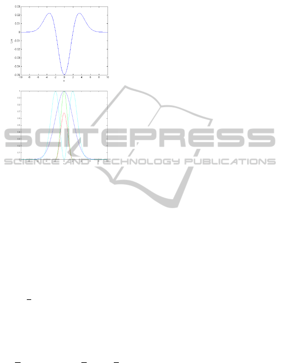
Figure 2: Second derivative L

of the plane model (σ

= 1)

at a scale σ = 1 (top) and Gauges for the density proﬁle of a

plane with σ

= 1 at a scale σ = 1 (blue): R

(red), S (cyan)

and plane strength P (green). The proﬁle across the plane, S

and P are normalized in the range [0, 1]. R

keeps the scale

relative to S.

in the volume may generate false positives. However,

the background usually has a density level different

from that shown by the structures of interest. A strat-

egy based on a density threshold t

(Fernandez and Li,

2005) helps to get rid of these false positives.

Local structures resembling ‘density steps’ in the

volume also make the gauge R produce a false peak.

A suitable detector for a local step is the edge

saliency (Lindeberg, 1998):

S = L

+ L

(5)

where L

∂I

∂i

∀i ∈ (x,y,z). A plane exhibits a high

value of S at the extremes and a low value at the centre

(Fig. 2(bottom)). Based on their response to a plane,

the ratio between the squared second-order and ﬁrst-

order derivatives (i.e. R

/S) quantiﬁes how well the

local structure around a voxel ﬁts the plane model and

not a step. We thus deﬁne plane strength as:

P =

(

,(L > t

) and



sign



∂R

∂r



6= sign



∂S

∂r



0 , otherwise

(6)

The ﬁrst condition in Eq. (6) denotes the density

thresholding described above. The second condition

represents the requirement that the slopes of R and

S in the gradient direction must have opposite signs.

This condition is important to restrict the response of

that function for steps (see Fig. 2(bottom)) . If the

local structure approaches the plane model, P will

have high values around the centre of the plane (high

values of R

, low values of S).

2.4 Hysteresis Thresholding and Global

Analysis

Due to the local nature of the plane model (see Sub-

section 2.1), any detector based on this model can also

generate a high response for structures different from

planar structures. For that reason, it is important to

incorporate “global information” to discern true pla-

nar structures from these others. The stages in this

subsection are introduced for this purpose.

First, thresholding is applied to P in order to dis-

card voxels unlikely belonging to planar structures.

Hysteresis thresholding has been shown to outper-

form the standard thresholding algorithm (Sandberg,

2007). Here two thresholds are used, the large valuet

undersegments the volume whereas the other t

over-

segments it. Starting from the undersegmented vol-

ume (seed voxels), adjacent voxels are added to the

segmented volume by progressively decreasing the

threshold until the oversegmenting level t

is reached.

Here we have increased the robustness of hystere-

sis thresholding by constraining the selection of seeds

to the particular characteristics of planar structures

in experimental biomedical datasets, namely the rela-

tively high number of voxels connected. So, we have

introduced two additional thresholds so that seed vox-

els belonging to components with less than t

pixels

slicewise, or t

in 3D, are discarded. This allows iso-

lation of seeds that are most representative of planar

structures, thus improving the global performance.

Finally, a global analysis stage intends to iden-

tify the segmented components that are actually pla-

nar structures. A distinctive attribute is their relatively

large dimensions. Therefore, the size (i.e. the num-

ber of voxels of the component) can serve as a ma-

jor global descriptor. A threshold t

(similar or equal

to t

) is then introduced to set the minimal size for a

component to be considered as a planar structure.

3 EXPERIMENTAL RESULTS

To illustrate the performance of the algorithm, it was

tested with several volumes taken under different ex-

perimental conditions and with several bioimaging

VISAPP 2012 - International Conference on Computer Vision Theory and Applications

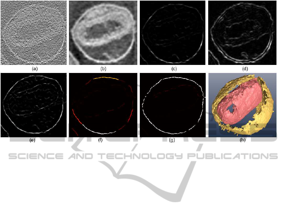
Figure 3: The procedure applied to a volume of Vaccinia virus obtained by electron tomography. (a) slice of the original

volume. (b) at a scale σ = 3. (c-e) R, S and P, respectively. (f, g) hysteresis thresholding. seed voxels to extract the outer

membrane after the t

and after t

thresholding, respectively. brighter colour means larger number of connected voxels. (h)

Membranes detected after the global analysis. The membrane of the internal core (in pink) was obtained after running the

algorithm at a scale of σ = 6.

techniques. The volumes were rescaled to a common

density range of [0, 1]. The optimal results were ob-

tained using the same basic parameter conﬁguration

for hysteresis thresholding, in particular t

∈[0.35,1],

∈ [0.05,0.4] and t

∈ [15, 35]. The values of the

parameters σ, t

, t

and t

, however, depend on the

speciﬁc dataset and were readily set by inspection of

the volume. σ is the thickness of the sought planes,

which were membranes in most of our tests.

First, to show the procedure at work, Fig. 3 shows

the different stages applied to a volume of Vaccinia

virus (Cyrklaff et al., 2005). This volume was ob-

tained by electron tomography under low electron

dose and cryogenic temperatures, which makes it par-

ticularly noisy and with low contrast. The algorithm

succeeds in segmenting both the outer and the inter-

nal core membrane by properly tuning the parame-

ter σ. A scale of σ = 3 was applied to extract the

outer membrane. For the core membrane, however, a

much higher value was necessary (σ = 6) because this

membrane actually comprises two layers that make it

rather thick, thereby needing a higher scale to extract

it separately.

Fig. 3(c-e) (which were obtained at σ = 3, tar-

geting at the outer membrane) clearly shows that,

though the gauge R actually quantiﬁes the level of

local membrane-ness, it still depends on the density

level. Thus, there are some parts of the membrane

where R exhibits weak values. On the contrary, P

only contains differential information and, therefore,

higher strength is shown throughoutthe membrane re-

gardless of the density value. However, the side ef-

fect is that other structures resembling planes at local

level also produce a high value of P (for instance, the

dense material between the outer membrane and the

core seen at the top of (e); or the ﬁber attached to the

internal side of the outer membrane seen at the bottom

of (e)). The hysteresis thresholding procedure and the

global analysis then manage to extract the true mem-

branes. This behaviour is an inherent feature of the

algorithm.

To further illustrate the performance of the algo-

rithm, it was applied to several volumes obtained by

electron tomography and using experimental condi-

tions that provides better contrast than in the pre-

vious case. The volumes contained different spec-

imens, namely vesicles, mitochondrion and chloro-

plast, respectively. Fig. 4 shows a gallery of the

structures, mostly membranes, detected by the algo-

rithm. The algorithm was run at a scale σ of 2,

1.5 and 0.1, respectively. As shown, all the planar

structures present in the volumes were clearly iden-

tiﬁed and come out of the background. The datasets

were taken from the CCDB (Cell-Centered DataBase,

http://ccdb.ucsd.edu) (Martone et al., 2008).

Finally, in order to demonstrate the applicabil-

SEGMENTATION OF PLANAR STRUCTURES IN BIOIMAGING

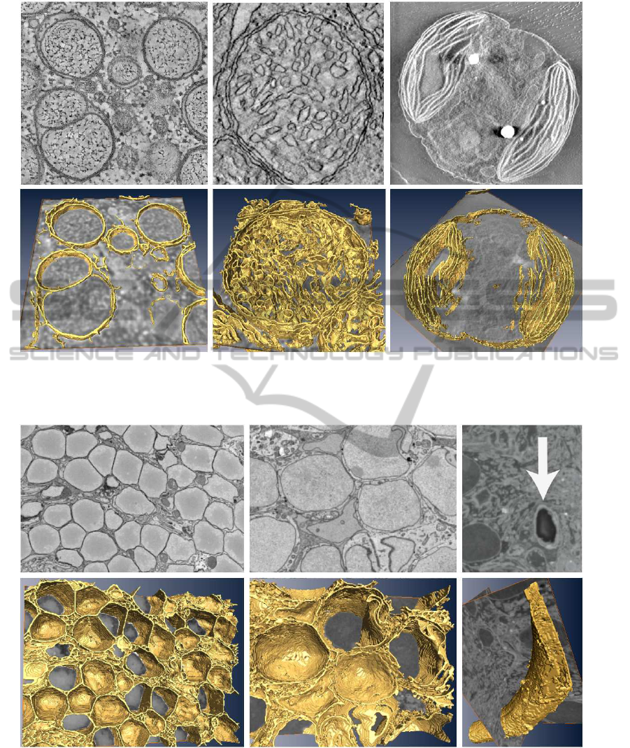
Figure 4: Planar structures detected by the algorithm for three different volumes containing vesicles, mitochondrion and

chloroplast, respectively, that were obtained by electron tomography. Top: a slice of the original volume is shown. Bottom:

3D visualization.

Figure 5: Planar structures detected by the algorithm for three representative areas of a thick retina tissue. Top: a slice of the

original volume is shown. Bottom: 3D visualization of the planar structures.

ity of the algorithm to other bioimaging disciplines,

we applied it to a volume derived from a study con-

sisting in the ultrastructural characterization of the

mouse optic nerve head and retina (Kim et al., 2010;

Nguyen et al., 2011), which was taken from the

CCDB database (Martone et al., 2008). In this study,

the thick tissue section was subjected to 3D recon-

struction by a technique known as ’Serial Block Face

VISAPP 2012 - International Conference on Computer Vision Theory and Applications

SEM’ (SBFSEM). Here the tissue is progressively

sliced into thin sections and the face of the remain-

ing block is imaged by means of a Scanning Elec-

tron Microscope (SEM). At the end of the process,

the images that were taken are stacked into a single

volume, hence the 3D reconstruction. The tissue that

was studied here contained different nerve cell lay-

ers. Figure 5 shows a gallery of representative areas

of the different layers, where the segmentation of the

planar structures performed by our algorithm is appar-

ent. For these cases, the scale used in the application

of the algorithm was 0.5.

4 CONCLUSIONS

We have presented a procedure to detect planar struc-

tures in volumes obtained by different bioimaging

techniques. It relies on a simple local model for a

plane and on the local differential structure to deter-

mine points whose neighbourhood resembles plane-

like features. Later stages of the algorithm then intend

to deﬁnitely determine which of those points do actu-

ally constitute the planar structures. The performance

of algorithm has been shown on a set of representative

volumes. In general, the algorithm has turned out to

be effective to detect planar structures, often found in

biological datasets. Therefore, it has potential to be a

useful tool for (semi-)automated interpretation of 3D

volumes obtained by different bioimaging technolo-

gies.

ACKNOWLEDGEMENTS

Work supported by grants MCI-TIN2008-01117 and

JA-P10-TIC6002. A.M.S. is a fellow of the Spanish

FPI programme.

REFERENCES

Chandler, D. and Roberson, R. W. (2009). Bioimaging:

current techniques in light and electron microscopy.

Jones and Barlett Pub.

Cyrklaff, M., Risco, C., Fernandez, J. J., Jimenez, M. V.,

Esteban, M., Baumeister, W., and Carrascosa, J. L.

(2005). Cryo-electron tomography of vaccinia virus.

Proc. Natl. Acad. Sci. USA, 102:2772–2777.

Fernandez, J. J. and Li, S. (2003). An improved algorithm

for anisotropic diffusion for denoising tomograms. J.

Struct. Biol., 144:152–161.

Fernandez, J. J. and Li, S. (2005). Anisotropic nonlinear

ﬁltering of cellular structures in cryoelectron tomog-

raphy. Comput. Sci. Eng., 7(5):54–61.

Florack, L. J., Romeny, B. H., Koenderink, J. J., and

Viergever, M. A. (1992). Scale and the differential

structure of images. Image and Vision Computing,

10:376–388.

Frangi, A., Niessen, W., Vincken, K., and Viergever, M.

(1998). Multiscale vessel enhancement ﬁltering. Lec-

ture Notes in Computer Science, 1496:130–137.

Frank, J., editor (2006). Electron tomography. Springer.

Kim, K., Ju, W., Hegedus, B., Gutmann, D., and Ellisman,

M. (2010). Ultrastructural characterization of the op-

tic pathway in a mouse model of neuroﬁbromatosis-1

optic glioma. Neuroscience, 170:178–188.

Koenderink, J. J. (1984). The structure of images. Biol.

Cybern., 50:363–370.

Lindeberg, T. (1990). Scale-space for discrete signals. IEEE

Trans. PAMI, 12(3):234–254.

Lindeberg, T. (1998). Edge detection and ridge detection

with automatic scale selection. Int. J. Computer Vi-

sion, 30:117–154.

Lucic, V., Forster, F., and Baumeister, W. (2005). Struc-

tural studies by electron tomography: from cells to

molecules. Ann. Rev. Biochem., 74:833–865.

Martinez-Sanchez, A., Garcia, I., and Fernandez, J. (2011).

A differential structure approach to membrane seg-

mentation in electron tomography. J. Struct. Biol.,

175:372–383.

Martone, M., Tran, J., Wong, W. W., Sargis, J., Fong, L., ans

S. P. Lamont, S. L., Gupta, A., and Ellisman, M. H.

(2008). The cell centered database: An update on

building community resources for managing and shar-

ing 3D imaging data. J. Struct. Biol., 161:220–231.

Nguyen, J., Soto, I., Kim, K., Bushong, E., Oglesby, E., Va-

liente, F., Yang, Z., Davis, C., Bedont, J., Son, J., Wei,

J., Ellisman, M., and Marsh, N. (2011). Myelination

transition zone astrocytes are constitutively phago-

cytic and have synuclein dependent reactivity in glau-

coma. Proc. Natl. Acad. Sci. USA, 108:1176–1181.

Sandberg, K. (2007). Methods for image segmentation

in cellular tomography. Methods in Cell Biology,

79:769–798.

Volkmann, N. (2010). Methods for segmentation and in-

terpretation of electron tomographic reconstructions.

Methods Enzymol., 483:31–46.

Witkin, A. P. (1983). Scale-space ﬁltering. In Proc. 8th Intl.

Conf. Artif. Intell., pages 1019–1022.

Young, I. T. and van Vliet, L. J. (1995). Recursive imple-

mentation of the gaussian ﬁlter. Signal Processing,

44:139–151.

SEGMENTATION OF PLANAR STRUCTURES IN BIOIMAGING