
IMPROVEMENT OF MOTION ESTIMATION BY ASSESSING
THE ERRORS ON THE EVOLUTION EQUATION
Isabelle Herlin
1,2
, Dominique Bereziat
3
and Nicolas Mercier
1,2
1
INRIA, Institut National de Recherche en Informatique et Automatique, Domaine de Voluceau, Rocquencourt BP 105,
78153 Le Chesnay, France
2
CEREA, Joint Laboratory ENPC - EDF R&D, Universit
´
e Paris-Est, 6-8 avenue Blaise Pascal, Cit
´
e Descartes,
Champs-sur-Marne, 77455 Marne la Vall
´
ee, France
3
UPMC, Universit
´
e Pierre et Marie Curie, 4 Place Jussieu 75005 Paris, France
Keywords:
Optical Flow, Data Assimilation, Optimal Control.
Abstract:
Image assimilation methods are nowadays widely used to retrieve motion from image sequences with heuris-
tics on the underlying dynamics. A mathematical model on the temporal evolution of the motion field has to
be chosen, according to these heuristics, that approximately describes the evolution of the velocity at a pixel
over the sequence. In order to quantify this approximation, we add an error term in the evolution equation
of the motion field and design a weak formulation of 4D-Var image assimilation. The designed cost function
simultaneously depends on the initial motion field and on the error value at each time step. The BFGS solver
performs minimization to retrieve both motion field and errors. The method is evaluated and quantified on
twin experiments, as no ground truth would be available for real data. The results demonstrate that the motion
field is better estimated thanks to the error control.
1 INTRODUCTION
Motion estimation from an image sequence is one ma-
jor issue of Image Processing in a large range of ap-
plicative domains. This allows for instance to study
the dynamics of clouds and estimate the ocean sur-
face circulation on satellite data. The retrieved mo-
tion fields can be further used as pseudo-observations
for 3D models.
In the Image Processing literature, motion fields
are most often inferred from an equation describ-
ing the transport of pixel brightness by velocity (for
instance the optical flow constraint equation used
in (Horn and Schunk, 1981) and (Isambert et al.,
2008), or the mass conservation equation of (B
´
er
´
eziat
et al., 2000). By nature, this transport equation
is under-constrained to retrieve the two components
of motion on 2D image data and spatial regulariza-
tion techniques are used to define a well-posed pro-
blem with a unique solution. This is the well-known
Tikhonov regularization, (Tikhonov, 1963).
However, heuristics on the dynamics displayed by
the image sequence are often available and should be
used to solve the problem of retrieving motion fields
from image data. The first concern is to select the ma-
thematical equations that optimally describe that dy-
namics. The second one is to define the process of
motion estimation from these equations and from the
links between the evolution of image values and the
motion field. Variational data assimilation methods,
and in particular 4D-Var methods, are emerging tech-
niques in the Image Processing community that al-
low this retrieval of motion from images, (Papadakis
et al., 2007), (Titaud et al., 2010) and (B
´
er
´
eziat and
Herlin, 2011)). These 4D-Var methods solve a system
of three equations that describes the temporal evolu-
tion of the state vector, the links between the observa-
tion values and state vector, and the background value
of the state vector. The name “background” comes
from the data assimilation community and refers to
the value given to the state vector at the beginning of
the optimization process. The solution of this system
of equations is then formulated as the solution of an
optimization problem.
The first 4D-Var method, (Le Dimet and Tala-
grand, 1986), supposes that the state vector evolution
equation has no error and perfectly describes the dy-
namics: the model is a Perfect Model (PM). In that
case, the control variable is reduced to the initial value
of the state vector at the beginning of the studied tem-
235
Herlin I., Béréziat D. and Mercier N..
IMPROVEMENT OF MOTION ESTIMATION BY ASSESSING THE ERRORS ON THE EVOLUTION EQUATION.
DOI: 10.5220/0003815802350240
In Proceedings of the International Conference on Computer Vision Theory and Applications (VISAPP-2012), pages 235-240
ISBN: 978-989-8565-04-4
Copyright
c
2012 SCITEPRESS (Science and Technology Publications, Lda.)

poral window, named assimilation window. The data
assimilation method is named strong 4D-Var.
Unfortunately, the heuristics that are available on
the dynamics of an image sequence are only appro-
ximating the reality. It is then valuable and wise
to assess that approximation by introducing an er-
ror in the evolution equation as in (Tr
´
emolet, 2006).
A weak formulation of 4D-Var, which includes such
error term ε(t) in the evolution equation, is exten-
sively described in (Valur H
´
olm, 2008). It is used to
solve image processing problems such as motion esti-
mation, (B
´
er
´
eziat and Herlin, 2011), or curve track-
ing, (Papadakis et al., 2005). The control variable
of the optimization problem becomes the state vec-
tor value over the whole assimilation window. The
incremental method used to solve the optimization
in (Valur H
´
olm, 2008) has however a major drawback:
it has a slow convergence compared to the steepest
gradient methods used for strong 4D-Var methods.
An alternative is to control the initial value of the state
vector and the error terms. The advantage is that it al-
lows an efficient minimization by the same methods
used for perfect models. This is applied for instance
in (Papadakis et al., 2007), even if authors do not dis-
cuss the impact on the results of including that error
term.
This paper analyses the advantages of adding an
error term ε(t) in the state vector dynamic equation
for the issue of motion estimation by image assimila-
tion and quantifies the impact on results. In Section 2
we define the state vector and the system of equations
used for image assimilation and motion estimation.
We introduce a pseudo-image component in the state
vector and justify its interest for image assimilation.
Section 3 describes the 4D-Var method that simul-
taneously controls the initial condition and the error
term ε(t) added to the evolution equation. Details on
the computation of the gradient of the cost function
are given in that section. Section 4 provides informa-
tion about the numerical implementation to allow du-
plication of the method by interested Readers. Twin
experiments are designed in Section 5 in order to eval-
uate quantitatively the impact of the error term on the
quality of estimated motion fields. This is the only
way to obtain a ground truth of the error involved in
the evolution equation. We last conclude in Section 6.
2 MATHEMATICAL SETTINGS
Let Ω, a rectangle of
2
, denote the bounded im-
age domain, [t
0
,t
N
] denote the temporal assimilation
window and define A = Ω × [t
0
,t
N
] the space-time
domain. We also denote H(Ω) the Sobolev space
included in L
2
(Ω), space of square-integrable func-
tion from Ω to . A location x ∈ Ω is defined as:
x =
x y
T
and the motion vector at location x and
date t ∈ [t
0
,t
N
] is written: w(x,t) =
u(x,t) v(x,t)
T
with u and v belonging to H
2
(Ω). Image observations
denoted Y(x,t) or I (x,t), according to the mathemat-
ical context of data assimilation or image processing,
are available.
As explained in the introduction, the motion es-
timation method relies on image assimilation. The
state vector has first to be defined. It includes
the two components u and v of the motion vector
w(x,t) and a pseudo-image I
s
(x,t) ∈ H
2
(Ω), which
has similar properties than the image observations:
the motion field transports the values of this pseudo-
image in the same way than image pixels. The
state vector is then defined as the function X(x,t) =
w(x,t)
T
I
s
(x,t)
T
. Having included the pseudo-
image I
s
, within the state vector, allows an easy com-
parison to the image observations at each acquisition
date: they have to be almost identical or their differ-
ence should be almost zero.
The heuristics on dynamics used in this paper is
the Lagrangian constancy of velocities:
dw
dt
=
∂w
∂t
+ (w
T
∇)w = 0 (1)
Being generic enough, this Lagrangian constancy is
a rough approximation that is usable for many image
data types (B
´
er
´
eziat and Herlin, 2011). The pseudo-
image I
s
obeys to the same heuristics than the image
data: the velocity field transports it:
∂I
s
∂t
+ w
T
∇I
s
= 0 (2)
Equations (1) and (2) only being heuristics, they
approximate the reality. An error term, ε(x,t) =
ε
w
(x,t)
T
ε
I
s
(x,t)
T
, is added to represent this un-
certainty and the evolution equation of the state vector
is then summarized by:
∂X
∂t
+ (X) = ε (3)
As the motion value is estimated from the image
observations, denoted Y(x,t), an observation equa-
tion is required to link the state vector to these ob-
servation data:
X = Y + ε
R
(4)
The observation operator projects the state vector
into the space of observations. As the state vector in-
cludes the pseudo-image component, reduces to:
X = I
s
. The observation error ε
R
(x,t) models the
acquisition noise of the image observations.
VISAPP 2012 - International Conference on Computer Vision Theory and Applications
236
During the motion estimation process, Eqs. (1)
and (2) are integrated in time. This requests an initial
value of the state vector at date t
0
. Some knowledge
of this value is often available and named the back-
ground X
b
(x). However, the state vector at date t
0
is not exactly equal to that background value and an
error term ε
B
(x) is introduced:
X(x,t
0
) = X
b
(x) + ε
B
(5)
The error variables ε, ε
R
and ε
B
are supposed un-
biased, Gaussian and characterized by their respective
covariance matrices Q, R and B.
For retrieving motion from the image observa-
tions, the equations (3), (4) and (5) must be simul-
taneously solved. In this paper, this is achieved with
the 4D-Var method described in the next section.
3 CONTROL OF MODEL ERROR
The data assimilation system obtained with
Eqs. (3, 5, 4) is written as:
∂X
∂t
+ (X) = ε (6a)
X(t
0
) = X
b
+ ε
B
(6b)
X = Y + ε
R
(6c)
Looking for the solution X that solves Sys-
tem (6a,6b,6c) is expressed as an optimization prob-
lem. A cost function is defined that has to be mini-
mized by controlling ε and ε
B
:
J[ε
B
,ε] =
1
2
Z
t
D
ε(t),Q
−1
ε(t)
E
+
1
2
D
ε
B
,B
−1
ε
B
E
(7)
+
1
2
Z
t
D
X(t) −Y(t),R
−1
[ X(t) − Y(t)]
E
h
,
i
denotes the space integral over the domain Ω. The
first term comes from Eq. (3), the second from Eq. (5)
and the third from Eq. (4). They express that the three
error terms have to be minimized, accordingly to their
respective covariance matrices Q, B and R.
In order to minimize the cost function J, its gradi-
ent is derived with calculus of variation.
Theorem 1. The gradient of J is given by:
∂J
∂ε(t)
[ε,ε
B
] = Q
−1
ε(t) + λ(t)
∂J
∂ε
B
[ε,ε
B
] = B
−1
ε
B
+ λ(t
0
)
with λ(t) the adjoint variable computed backward in
time by:
λ(t
N
) = 0 (8a)
−
∂λ(t)
∂t
+
∂
∂X
∗
λ(t) =
T
R
−1
× (8b)
[ X(t) − Y(t)]
Proof. The state vector and the functional J depend
on ε(t) (defined in Eq. (3)) and ε
B
(defined in Eq. (5)).
Let δJ and δX be the perturbations on J and X ob-
tained if ε(t) and ε
B
are respectively perturbed by
δε(t) and δε
B
. We obtain from Eq. (7):
δJ =
Z
t
δε(t),Q
−1
ε(t)
+
δε
B
,B
−1
ε
B
(9)
+
Z
t
δX(t),
T
R
−1
[ X(t) −Y (t)]
and from Eqs. (3) and (5):
∂δX(t)
∂t
+
∂
∂X
δX(t) = δε(t) (10a)
δX(t
0
) = δε
B
(10b)
Eq. (10a) gives, after multiplication by λ(t) and in-
tegration on the space-time domain, the following
equality:
Z
t
∂δX(t)
∂t
,λ(t)
+
Z
t
∂
∂X
δX(t),λ(t)
=
Z
t
h
δε(t),λ(t)
i
Integration by parts is applied on the first term and
the adjoint operator is used in the second one in order
to obtain:
−
Z
t
δX(t),
∂λ(t)
∂t
+ < δX(t
N
),λ(t
N
) >
− < δε
B
,λ(t
0
) > +
Z
t
δX(t),
∂
∂X
∗
λ(t)
=
Z
t
h
δε(t),λ(t)
i
(11)
From Eq. (8a), it comes that < δX(t
N
),λ(t
N
) > has a
null value. Eq. (8b) is then used to obtain:
−
δX(t),
∂λ(t)
∂t
+
δX(t),
∂
∂X
∗
λ(t)
=
< δX(t),
T
R
−1
[ X(t) −Y (t)] >
and Eq. (11) is rewritten as:
Z
t
< δX(t),
T
R
−1
[ X(t) −Y (t)] >=
< δε
B
,λ(t
0
) > +
Z
t
h
δε(t),λ(t)
i
From this and Eq. (9), we derive:
δJ =
Z
t
< δε(t),Q
−1
ε(t) > + < δε
B
,B
−1
ε
B
>
+ < δε
B
,λ(t
0
) > +
Z
t
h
δε(t),λ(t)
i
IMPROVEMENT OF MOTION ESTIMATION BY ASSESSING THE ERRORS ON THE EVOLUTION EQUATION
237

and obtain the gradient of J as given in Theorem 1:
∂J
∂ε(t)
[ε(t),ε
B
] = Q
−1
ε(t) + λ(t)
∂J
∂ε
B
[ε(t),ε
B
] = B
−1
ε
B
+ λ(t
0
)
The cost function J is minimized using an itera-
tive steepest descent method. At each iteration, the
forward time integration of X is performed and pro-
vides J, then a backward integration of λ computes
∇J. An efficient solver (Byrd et al., 1995), based on
the BFGS method, is used to perform the steepest de-
scent given J and ∇J.
4 NUMERICAL
IMPLEMENTATION
An explicit Euler scheme is applied to perform the
forward time integration of X. Time indexes go from
0 to N
t
for the assimilation window [t
0
,t
N
]. Moreover
a robust numerical scheme is proposed to discretize
in space. Eq. (1) is replaced by a system of two equa-
tions respectively describing the evolution of compo-
nents u and v of the velocity:
∂u
∂t
+ u
∂u
∂x
+ v
∂u
∂y
= 0 (12)
∂v
∂t
+ u
∂v
∂x
+ v
∂v
∂y
= 0 (13)
Each equation contains a linear advection part and a
non linear one. A source splitting, (Wolke and Knoth,
2000), is first applied on each equation and illustrated
on Eq. (12). Given an interval [t
1
,t
2
], the two follow-
ing equations are integrated independently:
∂u
∗
∂t
+ u
∗
∂u
∗
∂x
= 0 t ∈ [t
1
,t
2
] (14)
∂u
∗∗
∂t
+ v
∂u
∗∗
∂y
= 0 t ∈ [t
1
,t
2
] (15)
with u
∗
(x,y,t
1
) = u
∗∗
(x,y,t
1
) = u(x,y,t
1
). u(x,y,t
2
)
is then approximated as u(x,y,t
2
) = u
∗∗
(x,y,t
2
) +
(u
∗
(x,y,t
2
) − u
∗
(x,y,t
1
)).
The linear advection of Eq. (15) is approxi-
mated by a first order up-wind scheme, (Hundsdor-
fer and Spee, 1995). The non linear advection of
Eq. (14) is first rewritten in a conservative form,
∂u
∂t
+
∂
∂x
1
2
u
2
= 0, and approximated by a first or-
der Godunov scheme, (LeVeque, 1992).
The backward time integration of the adjoint vari-
able involves the adjoint operator
∂
∂X
∗
(Eq. (8b))
that is obtained thanks to an automatic differentiation
software, (Hasco
¨
et and Pascual, 2004).
5 EXPERIMENTS AND RESULTS
Two algorithms have been implemented and com-
pared during the experimental phase in order to
demonstrate the improvement provided by the ad-
ditional error term in the evolution equation. The
first one, named IM for Imperfect Model, relies on
Eqs. (3,4,5) with the error term ε(t) included in the
evolution equation of the state vector. The second
one, named PM for Perfect Model, satisfies the same
equations, but the error term is suppressed in Eq. (3).
The first term of the cost function J in Eq (7) vanishes
for PM and minimization is then only controlled by
ε
B
.
We designed a series of twin experiments for as-
sessing the impact of the error term ε(t). Three of
them are described in the following.
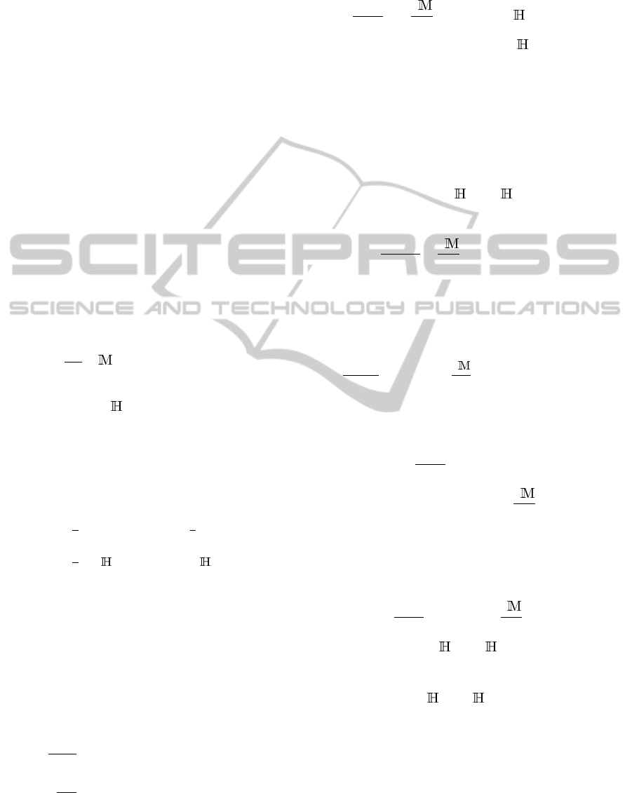
Given initial conditions, at index 0, on velocity
and pseudo-image (w
ref
(0),I
s
(0))
T
, as displayed in
Figure 1, and given a model error ε
ref
, Eq. (3) is in-
tegrated in time. We consider the snapshots of the
Figure 1: Initial conditions of the velocity field and pseudo-
image.
pseudo-image function, obtained by the simulation
at given indexes k
i
, to define the image observations
used in the assimilation experiments. In that way, we
have full knowledge of the initial motion field w
ref
(0)
and of the error values ε
ref
(t) that produce the obser-
vations and we can quantitatively compare them with
the results of the assimilation method obtained by IM
and PM.
The background value, X
b
=
w
b
,I
sb
T
, in Eq. (5),
is the same for IM and PM. The pseudo-image I
s
b
(x)
is chosen as the first observation denoted Y(x,k
1
).
For these experiments, we choose w
b
(x) =
~
0. As we
do not want to constrain w(0) to stay close to
~
0 dur-
ing the optimization process, the background term of
J, in Eq. (7), reduces to
D
ε
B
I
s
,B
−1
I
s
ε
B
I
s
E
. We empiri-
cally set B
I
s
and R to 1 for IM and PM. For IM, Q is a
2 × 2 diagonal matrix whose coefficients, Q
u
and Q
v
have small values. We use five image observations.
The discrete assimilation window has indexes from 0
to N
t
= 83 and observation images are available at in-
VISAPP 2012 - International Conference on Computer Vision Theory and Applications
238
dexes k
1
to k
5
= 1, 21, 41, 61 and 81.
Experiment 1. We first assess the results of IM in
the case where the error value ε(t) ≡
~
0 during the sim-
ulation that creates the observation images. Questions
are the following. IM being designed to estimate an
error value, will it be able to correctly estimate that
error with a null value? Being designed with no error
term, will PM obtain a better estimation of the real
motion field w
ref
(0) than IM?
The first observation is the initial condition of Fig-
ure 1 and the four next one are displayed on Figure 2.
Figure 2: First Experiment. Observation Images.
A qualitative and quantitative comparison of the
initial motion fields retrieved by PM, w
PM
(0), and
IM, w
IM
(0), with the ground truth, w
ref
(0), is
achieved. Figure 3 displays these three velocity fields.
They are visually identical: both PM and IM cor-
rectly estimate motion. To quantitatively compare a
(a) w
ref
(0). (b) w
PM
(0). (c) w
IM
(0).
Figure 3: First Experiment. Comparison of the estimations
with ground truth.
velocity result w with the ground truth w
ref
at index
0, average and standard deviation of the absolute an-
gular error |θ − θ
ref
| and the relative norm difference
(kw − w
ref
k/kw
ref
k) are measured. These values are
provided in Table 1 for PM and IM. This confirms that
the two methods compute a correct velocity field with
a mean angular inaccuracy less than 1 degree and an
average of the relative norm difference around 2%. In
conclusion, the presence of the error term ε(t) has no
negative impact if the observation data have been pro-
duced without adding error in the evolution equation
during the simulation process.
Experiment 2. In that experiment, the error term,
ε
ref
(t), used during the simulation of the image obser-
vations, has a constant value over the space-time do-
main. To study separately the errors on the dynamics
(motion components) and on the pseudo-image, we
constrain the temporal evolution of the pseudo-image
Table 1: First Experiment. Statistics on the inaccuracy of
the motion fields estimated by PM and IM at index 0.
|θ − θ
ref
| kw − w
ref
k/kw
ref
k
Method mean st. dev. mean st. dev.
PM 0.82 2.24 0.018 0.046
IM 0.79 2.11 0.023 0.046
to be perfect and exactly satisfy the transport equa-
tion. We set ε
ref
(t)(x) =
10
−3
10
−3
0
T
. The
value 10
−3
corresponds to a final cumulative error of
70% of the maximum of the initial velocity norm.
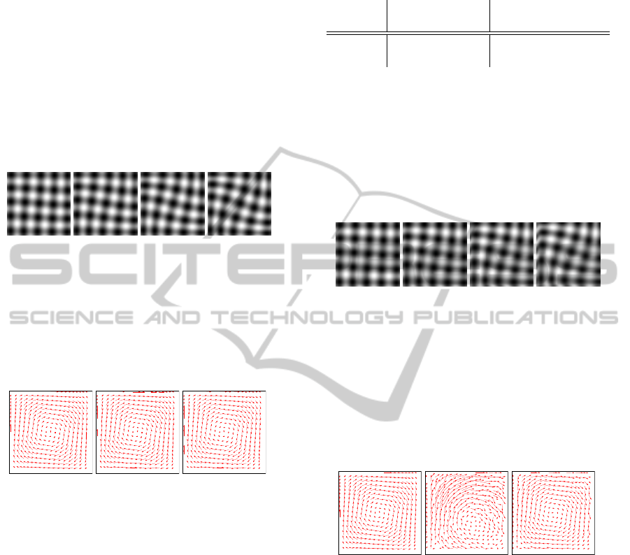
The first observation is the initial condition (Fig-
ure 1) and the four next ones are obtained by integrat-
ing Eq. (3) (see Figure 4).
Figure 4: Second Experiment. Observations Images.
Results are displayed on Figure 5. As it can be
seen, only IM computes a correct velocity field while
PM completely fails due to the noise included during
the simulation that produces the observations. PM,
relying on a perfect evolution equation, is unable to
retrieve the correct solution and computes the initial
velocity field that is the best compromise between
the evolution model and the observations. Table 2
(a) w
ref
(0). (b) w
PM
(0). (c) w
IM
(0).
Figure 5: Second Experiment. Comparison of the estima-
tions with ground truth.
provides statistics on the difference between the mo-
tion results and the ground truth: it confirms that IM
significantly improves the motion estimation both in
norm and in direction, due to the error term added in
the evolution equation.
Experiment 3. In that experiment, ε
ref
(t), used dur-
ing the simulation of the image observations, is con-
stant in space and random in time. We consider a
Gaussian noise with a variance of 10
−5
for both com-
ponents u and v.
The first observation is the initial condition of Fig-
ure 1 and the four next one are displayed on Figure 6.
As in the first experiment, the initial motion fields re-
IMPROVEMENT OF MOTION ESTIMATION BY ASSESSING THE ERRORS ON THE EVOLUTION EQUATION
239

Table 2: Second Experiment. Statistics on the inaccuracy of
the motion fields estimated by PM and IM at index 0.
|θ − θ
ref
| kw − w
ref
k/kw
ref
k
Method mean st. dev. mean st. dev.
PM 24.16 30.34 0.32 0.44
IM 5.98 11.40 0.11 016
Figure 6: Third Experiment. Observations Images.
trieved by PM and IM are qualitatively similar to the
ground truth. Table 3 gives statistics on the difference
between the results and the ground truth. It shows
that both methods estimate correctly the velocity with
a slight advantage to IM.
Table 3: Third Experiment. Statistics on the inaccuracy of
the motion fields estimated by PM and IM at index 0.
|θ − θ
ref
| kw − w
ref
k/kw
ref
k
Method mean st. dev. mean st. dev.
PM 6.91 10.14 0.13 0.57
IM 5.34 8.09 0.10 0.48
6 CONCLUSIONS
This paper discusses a data assimilation method that
simultaneously estimates motion from image data
and the inaccuracy in the evolution equation used to
model the dynamics of that motion field. For that pur-
pose, an error term is added to the evolution equation,
which is part of the data assimilation system, and con-
trolled by the optimization method. As a result, the
method provides the motion field and the error value
on the dynamics at each time step of the assimilation
window.
The method, named IM as Imperfect Model, has
been quantified on twin experiments and compared
with a Perfect Model, named PM, that does not in-
volve the error term. All experiments showed that IM
better estimates motion if the dynamics is not accu-
rately described by the evolution equation: an error
term has been added during the synthesis of image
observations. The improvement obtained with IM is
clearly visible in the second experiment that presents
a large deviation of the real dynamics to the evolution
equation. In that case, the perfect model PM com-
pletely fails to retrieve the motion field. This is clearly
visible when motion results are displayed. In all other
experiments, a quantitative improvement is obtained
with the Imperfect Model, if the simulation creating
the image observations included some error.
An important perspective of that research work
would be, for instance, the detection of changes of
dynamics over long temporal sequences.
REFERENCES
B
´
er
´
eziat, D. and Herlin, I. (2011). Solving ill-posed image
processing problems using data assimilation. Numer-
ical Algorithms, 56(2):219–252.
B
´
er
´
eziat, D., Herlin, I., and Younes, L. (2000). A general-
ized optical flow constraint and its physical interpre-
tation. In CVPR, pages 487–492.
Byrd, R. H., Lu, P., and Nocedal, J. (1995). A limited
memory algorithm for bound constrained optimiza-
tion. Journal on Scientific and Statistical Computing,
16(5):1190–1208.
Hasco
¨
et, L. and Pascual, V. (2004). Tapenade 2.1 user’s
guide. Technical Report 0300, INRIA.
Horn, B. and Schunk, B. (1981). Determining optical flow.
Artificial Intelligence, 17:185–203.
Hundsdorfer, W. and Spee, E. (1995). An efficient hori-
zontal advection scheme for the modeling of global
transport of constituents. Monthly Weather Review,
123(12):3,554–3,564.
Isambert, T., Berroir, J., and Herlin, I. (2008). A multi-
scale vector spline method for estimating the fluids
motion on satellite images. In ECCV, pages 665–676.
Springer.
Le Dimet, F.-X. and Talagrand, O. (1986). Variational al-
gorithms for analysis and assimilation of meteorologi-
cal observations: Theoretical aspects. Tellus, 38A:97–
110.
LeVeque, R. (1992). Numerical Methods for Conservative
Laws, chapter Godunov’s method. Lectures in Math-
ematics. ETH Z
¨
urich, Birkha
¨
user Verlag, 2nd edition.
Papadakis, N., Corpetti, T., and M
´
emin, E. (2007). Dy-
namically consistent optical flow estimation. In ICCV,
pages 1–7.
Papadakis, N., M
´
emin, E., and Cao, F. (2005). A variational
approach for object contour tracking. In ICCV work-
shop on variational, geometric and level set methods
in computer vision, pages 259–270.
Tikhonov, A. N. (1963). Regularization of incorrectly posed
problems. Soviet mathematics - Doklady, 4:1624–
1627.
Titaud, O., Vidard, A., Souopgui, I., and Le Dimet, F.-X.
(2010). Assimilation of image sequences in numerical
models. Tellus A, 62:30–47.
Tr
´
emolet, Y. (2006). Accounting for an imperfect model in
4D-Var. Quaterly Journal of the Royal Meteorological
Society, 132(621):2483–2504.
Valur H
´
olm, E. (2008). Lectures notes on assimilation algo-
rithms. European Centre for Medium-Range Weather
Forecasts Reading.
Wolke, R. and Knoth, O. (2000). Implicit-explicit Runge-
Kutta methods applied to atmospheric chemistry-
transport modelling. Environmental Modelling and
Software, 15:711–719.
VISAPP 2012 - International Conference on Computer Vision Theory and Applications
240
