
PITCH-SENSITIVE COMPONENTS EMERGE FROM
HIERARCHICAL SPARSE CODING OF NATURAL SOUNDS
Engin Bumbacher
1
and Vivienne Ming
2
1
School of Computer and Communication Science, EPFL, Lausanne, Switzerland
2
Socos LLC, San Francisco & Visiting Scholar, Redwood Center for Theoretical Neuroscience
U. C., Berkeley, U.S.A.
Keywords:
Pitch perception, Gist, Sparse coding, Generative hierarchical models, Gaussian mixture models, Bayesian
inference, Auditory processing, Speech processing.
Abstract:
The neural basis of pitch perception, our subjective sense of the tone of a sound, has been a great ongoing de-
bates in neuroscience.Variants of the two classic theories - spectral Place theory and temporal Timing theory -
continue to continue to drive new experiments and debates (Shamma, 2004). Here we approach the question
of pitch by applying a theoretical model based on the statistics of natural sounds. Motivated by gist research
(Oliva and Torralba, 2006), we extended the nonlinear hierarchical generative model developed by Karklin et
al. (Karklin and Lewicki, 2003) with a parallel gist pathway. The basic model encodes higher-order structure
in natural sounds capturing variations in the underlying probability distribution. The secondary pathway pro-
vides a fast biasing of the model’s inference process based on the coarse spectrotemporal structures of sound
stimuli on broader timescales. Adapting our extended model to speech demonstrates that the learned code de-
scribes a more detailed and broader range of statistical regularities that reflect abstract properties of sound such
as harmonics and pitch than models without the gist pathway. The spectrotemporal modulation characteristics
of the learned code are better matched to the modulation spectrum of speech signals than alternate models,
and its higher-level coefficients capture information which not only effectively cluster related speech signals
but also describe smooth transitions over time, encoding the temporal structure of speech signals. Finally, we
find that the model produces a type of pitch-related density components which combine temporal and spectral
qualities.
1 INTRODUCTION
Pitch is the subjective attribute of a sound’s funda-
mental frequency that is related to the temporal peri-
odicity of the waveform. As such, it refers to several
distinct percepts which include spectral pitch (evoked
by a single tone), periodicity pitch (evoked by har-
monic complex tones that are spectrally resolved by
the cochlea) and residue pitch (a low pitch associ-
ated with the periodicity of the total waveform of a
group of high harmonics - the residue - that are spec-
trally unresolved by the cochlea) (Shamma, 2004).
Both the periodicity and the residue pitch do not re-
quire energy at the fundamental frequency of the com-
plex tones (phenomenon of the missing fundamental).
There has long been a debate about the mechanisms
that give rise to these different pitch percepts, with
a classical distinction between the Place and Timing
theories (Griffiths et al., 1998). The traditional place
theories explain pitch perception in terms of the pat-
tern of excitation produced along the tonotopically or-
ganized basilar membrane. Pitch could then be com-
puted via template matching (Shamma, 2004). On the
other hand, time theories promote the idea that pitch is
related to the time pattern of neural activity across the
auditory nerve. A global pitch percept emerges from
the dominant periodicity computed from the activity
of the cochlear neurons phase-locked to the corre-
sponding individual harmonics of the sound complex
(Griffiths et al., 1998). In the case of periodicity pitch,
both theories are able to explain how the frequencies
of the harmonics are determined. When it comes to
residue pitch, the place theory fails to identify the
pitch of complex tones when there is no well-defined
spectral structure or when all the harmonics are unre-
solved (Griffiths et al., 1998), as opposed to the time
theory. In the course of time, physiological and psy-
chophysical research has collected evidence and de-
scribed phenomena supporting both theories. Oxen-
ham et al. (Oxenham et al., 2004) have recently con-
219
Bumbacher E. and Ming V. (2012).
PITCH-SENSITIVE COMPONENTS EMERGE FROM HIERARCHICAL SPARSE CODING OF NATURAL SOUNDS.
In Proceedings of the 1st International Conference on Pattern Recognition Applications and Methods, pages 219-229
DOI: 10.5220/0003786802190229
Copyright
c
SciTePress

ducted experiments whose results indicate that com-
plex sounds with identical temporal regularity could
produce different pitch percepts, which is strongly in
favor of the place theory. By contrast, Shannon et al.
(Shannon et al., 1995) showed that speech recogni-
tion is possible with only temporal cues, and work by
Griffiths (Griffiths et al., 1998) and Patterson (Patter-
son et al., 2002) indicates that pitch can be produced
without a set of harmonically related peaks in the in-
ternal spectrum.
As an alternative approach to analysing neural re-
sponse to stimuli, we looked directly at the statistical
structure of naturally occurring sounds, such as hu-
man speech, by means of an extended version of the
generative hierarchical model developed by Karklin
and Lewicki (2003, 2005) - the so-called density com-
ponent model. This model is a generalization of
linear efficient coding methods such as ICA (Bell
and Sejnowski, 1995) and sparse coding (Olshausen
and Field, 1996) in which the coefficients of the lin-
ear filters are no longer assumed to be independent.
Karklin and Lewicki (2003, 2005) have shown that
their model captures higher-order statistical regulari-
ties that reflect more abstract, invariant properties of
the signal. However, these statistical models are gen-
erally implemented such that the inference process is
based on randomly initialized stochastic gradient de-
scent methods of the maximum a posteriori approxi-
mations of the probability distributions. As the space
of the posterior probability distribution is highly non-
linear, the inference process is significantly affected
by its initialization, not only in terms of stability but
also in terms of the information captured by the in-
ferred coefficients. Hence, random initializations in-
troduce a systemic bias to the encoding stage, affect-
ing the learning process of the density components.
Here, we have extended the density component
model in order to address these shortcomings. First,
we replaced the lower layer with an overcomplete
sparse coding model, in line with studies of Lewicki
and Sejnowski (2000) showing that overcomplete rep-
resentations increase the efficiency of the code and its
flexibility to encode various signal structures. Sec-
ondly, we softened the pure bottom-up approach of
the encoding process by incorporating a pathway that
serves as the initialization step of the inference pro-
cess of the higher layer of the density component
model based on a coarse gist representation of the re-
spective sound segment. We refer to this pathway as
the gist pathway. As such, the gist pathway moves the
system into an appropriate - in terms of the gist repre-
sentation - region of the posterior probability distribu-
tion and thus eliminates the randomness of the former
initialization process. In other words, this pathway
acts as a predictive mapping of the sound segment
into the space of higher-order structural features, by
means of the gist information extracted from the seg-
ment itself.
Having applied the model to human speech sig-
nals, we show that the learned higher-level represen-
tations are strikingly different when the gist path-
way is implemented. They are significantly better
adapted to the modulation spectrum of the speech
signals. Furthermore, these higher-level representa-
tions incorporate several types of components that ac-
count for pitch-encoding that have not been reported
previously. These types encompass both harmonic
templates and units that combines both temporal and
spectral qualities. Derived from information theoretic
approaches alone, these units shed a new light on the
debate about the different mechanisms that give rise
to pitch perception. Finally, the inferred coefficients
not only enable intuitively meaningful clustering of
speech signals but also exhibit smooth transitions over
time, which can be used for further structural encod-
ing.
2 EXTENDED DENSITY
COMPONENT MODEL
The extended density component model is an hier-
archical generalization of the sparse coding model
(Olshausen and Field, 1996). It builds on the den-
sity component model of Karklin and Lewicki (2005),
but further incorporates an additional pathway as de-
scribed in section 2.1. Likewise, the data is assumed
to be generated as a combination of a set of linear ba-
sis functions a
i
. In matrix form,
x = Au +ε, (1)
where the a
i
are the columns of A, and u are the ba-
sis function coefficients. Assuming the noise ε to be
Gaussian, we get
p(x|A,u) ∝ exp
−
∑
i
1
2σ
2
ε
(x
i
−
∑
j
A
i j
u
j
)
2
!
. (2)
In our case, x are sound pressure waveforms of
human speech.
The standard efficient coding models assume the
basis function coefficients independently follow gen-
eralized Gaussian distributions with equal variances
λ,
p(u) =
∏
i
zexp
u
i
λ
q
, (3)
where z = q/(2λΓ(1/q)) is the normalizing constant
and λ is usually is fixed to one. However, the den-
sity component model goes a step further by capturing
ICPRAM 2012 - International Conference on Pattern Recognition Applications and Methods
220

the dependence among the linear coefficients through
their respective variances, thus accounting for local
deviations from the unit variance assumed by the stan-
dard models. It is assumed that the set of λ values can
be modeled with a linear combination of density com-
ponents B
dc
and coefficients v
dc
as follows:
λ = c exp(B
dc
v
dc
). (4)
We set q
i
= 1 for all i to model the linear coefficients
to be sparse; and with c =
p
Γ(1/q
i
)/Γ(3/q
i
) = 1 and
equation (4), equation (3) becomes
p(u|B
dc
,v
dc
) =
∏
i
1
2λ
i
exp
u
i
λ
i
. (5)
Thus, the logarithm of the joint prior distribution of
the coefficients u can be written as
−log p(u|B
dc
,v
dc
) ∝
∑
i j
B
dc,i j
v
dc, j
+
+
∑
i
u
i
exp([B
dc
v
dc
]
i
)
(6)
(for derivation see appendix). Placing a sparse fac-
torable prior on the latent variables v
dc
,
p(v
dc
) =
∏
i
p(v
dc,i
) =
∏
i
exp
v
dc,i
µ
dc
, (7)
constrains them to independence, while independence
of the coefficients u is now conditioned on these
higher-level coefficients.
The probability density function for the linear
model (1) is obtained by marginalizing over the co-
efficients
p(x|A,B
dc
) =
Z
p(x|u,A)p(u|B
dc
)du
= p(u|B
dc
)/|detA| (8)
with
p(u|B
dc
) =
Z
p(u|B
dc
,v
dc
)p(v
dc
)dv
dc
. (9)
As calculating these integrals is computationally
intractable, we approximate them by their maximum
a posteriori (MAP) estimations which are calculated
by means of gradient descent algorithms.
To distinguish between the matrices A and B, we
will refer to the columns of A linear features or sparse
components (SC) and the columns of B
dc
density com-
ponents (DC).
2.1 Gist Pathway
As described in the introduction, the space of the
posterior probability distribution is highly nonlinear,
characterized by a vast number of local extrema. Due
to this nonlinearity, working with the maximum a pos-
teriori estimates of the coefficients makes the infer-
ence process very sensitive to the initialization, as the
gradient descent algorithm inherently only finds local
extrema. Thus, different randomly initialized infer-
ence runs for the same sound segment lead to different
inferred coefficients.
We have incorporated an initialization step of the
inference process of the density component coeffi-
cients that is entirely data-driven and hence determin-
istic. Motivated by research on gist (Oliva and Tor-
ralba, 2006) (Harding et al., 2007), we refer to the
initialization step as the gist pathway. While the pur-
pose of the sparse component layer is to establish an
accurate sparse representation of the initial signal it-
self, the gist pathway is designed to be a fast pro-
cessing step that extracts globally meaningful infor-
mation (gist) about the coarse spectrotemporal struc-
ture of the signal. For example, in the case of a signal
with predominant power in the high frequencies, the
gist pathway does not determine the single contribu-
tions of the sparse components, but rather captures the
overall characteristic - high pitch - and thus initializes
the inference process of the density component coef-
ficients v
dc
by favoring the density components that
best capture the corresponding frequency properties
of the signal.
Thus, in order to determine the gist of a given
sound pressure waveform x, the spectrogram of the
sound encompassing this segment and parts of the
preceding and the subsequent signal is computed and
projected into the space of the significant principal
components. This provides a coarse, phase-invariant
representation u
G
of the sound of interest. This works
well as the spectrogram is an estimate of the local
spatiotemporal power in a sound, which is therefore
related to the variance variables λ in the density com-
ponent model.
In the next step, the sound is further processed by
applying a sparse coding model on these projections
u
G
, based on the assumption that they can be written
as a linear superposition of gist basis functions B
G
:
u
G
= B
G
v
G
(10)
with a sparse set of coefficients v
G
. Thus, within the
standard sparse coding approach, under the assump-
tion of additive Gaussian noise, the cost function to
be minimized is given by the log-posterior probabil-
ity of the coefficients (similar to (2))
log p(v
G
|u
G
,B
G
) = log p(u
G
|v
G
,B
G
) + log p(v
G
)
∝ −
1
2σ
2
ε
ku
G
− B
G
v
G
k
2
−
∑
k
v
G,k
µ
G
(11)
PITCH-SENSITIVE COMPONENTS EMERGE FROM HIERARCHICAL SPARSE CODING OF NATURAL SOUNDS
221

Here, the distribution of the coefficients v
G
is mod-
eled as a Laplacian with uniform variance, as in equa-
tion (7). By setting the number of linear features
(columns of the matrix B
G
= [b
G,1
,b
G,2
,...,b
G,M
])
equal to the number of density components, the in-
ferred coefficients v
G
serve as the initialization to the
inference process of the higher-order coefficients B
dc
.
As the gist basis functions encode the activity of prin-
cipal components of the spectrogram of the sound on
a broader timescale than density components, the gist
pathway turns out to provide the density components
with additional information about the sound.
We predict that such a gist-modulated prior on the
v
dc
enables the second layer of the density component
model to encompass a broader range of structures of
the sound, as the gist pathway provides a robust rep-
resentation of the broad-scale sound, in addition to
the sparse components, and as such drives the system
towards a more likely representation of the sound sig-
nal.
Details to the inference process can be found in
the appendix.
3 METHODS
We provide results and analyses for the TIMIT speech
corpus (Garofolo et al., 1990), which includes a di-
verse group of native English speaker reading phonet-
ically diverse English sentences. The sampling rate
has been converted to 8kHz.
We have a two times overcomplete
1
set of sparse
components A, and 50 density components. The
length of the sound extracts T was set to be 20 ms.
This time length is on the same order of magnitude
as the temporal extent of formants and formant tran-
sitions (Harding et al., 2007) (Turner and Sahani,
2007). In order to remove second-order correlations,
the set of sounds has been whitened.
The MAP posteriors are estimated by means of
conjugate gradient descent software (Olshausen and
Field, 1997).
4 RESULTS
4.1 Density Components of the Fully
Extended Model
The density components presented in this section are
the results of training the fully extended density com-
1
Overcomplete with respect to the number of sample
points.
ponent model. In order to interpret the weights of a
density component, we first characterize each sparse
component as ellipses in the spectrotemporal domain.
Each ellipse is centered around the center of fre-
quency and center of the temporal envelope of the cor-
responding sparse component. The height and width
of each ellipse corresponds to the bandwidth and tem-
poral envelope of the component. We then color each
ellipse based on the weight of a given density com-
ponent. Patterns in the organization of the sparse
components revealed by this visualization show how
each density component captures meaningful depen-
dencies among the sparse components in the time-
frequency domain. The results are illustrated in figure
1.
We find that some of the density components
shown in figure 1 bear resemblance to the ones
Karklin and Lewicki (2005) reported (e.g. top row).
However, our use of a logarithmic frequency axis,
in accordance to the tonotopic organization of the
cochlea (Shamma, 2001), reveals more spectrotem-
poral interdependencies between the sparse compo-
nents. Such as the very specialized type of den-
sity components that encodes the phase-locking rela-
tionship between the amplitude modulation of mid-
and high-frequency linear features and very few low-
frequency linear features (figure 1 bottom row). The
possible role of these types of density components is
further discussed in the following subsection.
Representing the density components by the cen-
ters of mass of the modulation spectra of each den-
sity components allows us to characterize the pop-
ulation of density components. Thus, we can com-
pare the signal structure encoded by the population
of density components to the modulation spectra of
speech signals (Singh and Theunissen, 2003). The
spectrogram of a density component from which the
modulation spectrum is estimated was generated by
summing the spectrograms of each sparse component,
weighted by the corresponding weights of the higher-
level unit. The modulation spectrum for speech used
for the comparison is obtained from (Singh and The-
unissen, 2003). Singh et al. generated the spectro-
grams for human speech differently, but it is assumed
that this does not affect the conclusions that can be
drawn from a comparison. This allows to compare
the impact of different initializations of the inference
process.
In figure 2b, we overlaid the modulation spectrum
for speech
1
with the set of centers of mass of the mod-
ulation spectra for the density components, both for
1
We constrained ourselves to positive modulation fre-
quencies as a trade-off between resolution of the image and
completeness of information.
ICPRAM 2012 - International Conference on Pattern Recognition Applications and Methods
222
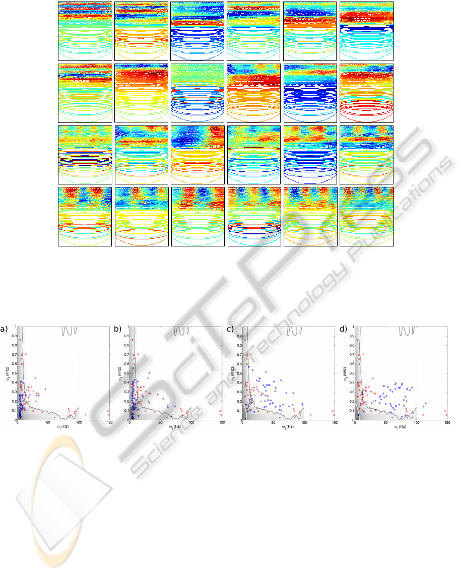
Figure 1: Subset of density components optimized for speech. Each squared figure corresponds to one of 24 density com-
ponents. Within such a square, each ellipse represents a sparse component in the spectrotemporal domain. The temporal
envelope width is divided in half for illustrational purposes. The ellipses are colored according to the weights in the particu-
lar density component. Red corresponds to significantly positive weights, and blue to significantly negative weights. Green
shaded colors stand for values close to zero. The time window is 20 ms, and the frequency axis encompasses 4 kHz on a
logarithmic scale. The density components are ordered according to their spectrotemporal modulation characteristics.
Figure 2: Population of modulation spectra of density components for different initializations. The centers of mass were
overlaid with the spectrograms of speech calculated by Singh and Theunissen (2003). The red squares are the population
of modulation spectra of density components for gist initialization, as a comparison. a) - c) show the results of optimizing
the model to speech when initializing the encoding process of the higher-order coefficients with random gaussian noise with
different variances σ. a) σ = 0.1. b) σ = 0.5. c) σ = 1.0. d) The coefficients were initialized based on the estimated local
variance of the projections of the data onto the linear features. See text for further information.
the hierarchical models with the gist pathway (red)
and without it (blue). We conclude that the density
components emerging from the hierarchical model in-
corporating the gist pathway are better adapted to the
spectrotemporal structure of speech. The blue dots
correspond to density components learned by initial-
izing the inference process either with random Gaus-
sian noise or with the local variance structure of the
linear filter outputs. First, the centers of mass are con-
centrated on regions of the speech modulation spec-
trum of high power. The frequency modulation fre-
quencies are smaller than 0.9 cycles/kHz, and those
of amplitude modulation are within the range of up
to 100Hz and beyond. Secondly, in speech signals as
well as the learned density components, high spectral
and high temporal modulations are unlikely to occur
at the same time, reflected by the star-shaped pattern
of the modulation spectrum. The modulation charac-
teristics of the other density components derived from
models without gist initialization are less well adapted
to the range of speech structures. They show signif-
icantly more redundancy than the ones with the gist
PITCH-SENSITIVE COMPONENTS EMERGE FROM HIERARCHICAL SPARSE CODING OF NATURAL SOUNDS
223

initialization or the ones based on initialization with
the local variance structure.
How well the density components are able to
generalize across natural signals can be assessed by
looking at how well the speech signals are clustered
based on the response patterns of the density compo-
nents. In figure 3, we apply Locally Linear Embed-
ding (LLE)
2
to the raw speech signals, the SC and
the DC coefficients. This method discovers structures
of high-dimensional data by assuming that it is sam-
pled from a smooth manifold, and thus creates natural
clusters of the data. As opposed to the raw data it-
self and sparse components, the output of the density
components captures similarities of sound segments
and separates distinct sound regions. The number of
neighbors chosen for the LLE algorithm did not affect
the quality of the results.
Furthermore, the clustering of the density com-
ponent coefficients within the two-dimensional pro-
jection additionally reflects the temporal structure of
the speech signal (not visualized in figure 3): Coef-
ficients representing samples at the beginning of the
sound segment are projected onto the left-hand side
of the projection space while those coding the signal
at later times are projected onto the right-hand side.
The coefficients representing the region of transition
are scattered in-between the two clusters, slowly tran-
sitioning from left to right. The temporal course of
the higher-level coefficients reflect the temporal struc-
ture of their stimuli through smooth changes. This is
also indicated by figure 4. We have applied a slid-
ing window to the same sound extract as used in fig-
ure 3 and inferred the coefficient values v
dc
at each
step. The population of these inferred coefficients v
dc
has been projected into the joint space of three spe-
cific density components, as shown in figure 4. Figure
4 reveals that the coefficient values are not scattered
randomly across the three-dimensional space but are
located on a clearly oval-like manifold. Furthermore,
when watching an animation that illustrates how the
coefficient values of these three components evolve
in the joint space when sliding the window across the
sound extract, one can observe that the coefficients
change smoothly over time.
4.1.1 Pitch Sensitivity
We found three types of pitch-related density com-
ponents. One set of components represents har-
monic relations among the sparse components as fre-
quency modulations, in accordance with the previous
2
”An unsupervised learning algorithm that computes a
low dimensional, neighborhood preserving embedding of
high dimensional data” (Saul and Roweis, 2000)
research (Klein et al., 2003), favoring the place the-
ory. Within a set of 50 density components, these
harmonicity units made up about 1/4 of the whole
set. The second set of components encodes pitch
by amplitude modulation across the mid- and high-
frequencies, with no distinct activation pattern in the
lower frequencies (type-I AM units), similar to the pe-
riodicity sensitive units from (Ming et al., 2009). The
units of Ming et al. (2009) emerged from applying a
sparse coding algorithm to the output of a pitch-based
auditory image model. The third type of density com-
ponents encodes the amplitude modulation across the
mid- and high-frequency sparse components phase-
locked to a low-frequency sparse component with a
center frequency matched to the corresponding mod-
ulation frequency (type-II AM units), as an analogue
to residue pitch. This is illustrated in figure 5.
Shown are three type-II AM units which capture
the relationship between the fundamental frequency
and the amplitude modulation in three different ways.
In figure 5a, the waveform of the linear feature with
center frequency 108.5 Hz alone synchronizes with
the phase-locked activity of the higher frequency-
units. Therefore, the density component assigns a sig-
nificantly positive weight to this low-frequency unit,
while all the neighboring units have negative weights.
Whenever the amplitude modulation frequency and
the phase of the modulation do not have a single
counterpart within the low-frequency sparse compo-
nents, the density component tries to encode the fun-
damental frequency by means of a combination of the
low-frequency units, as seen in figure 5b and c. The
higher-order unit of 5b has big positive weights on the
two low-level units with the smallest frequencies and
weights close to zero on their neighbors. The sum
of the waveforms of the two units, weighted accord-
ingly, matches the amplitude modulation. Similarly,
the density component in figure 5c has a big negative
weight on the low-level unit with a center frequency
of 108.7 Hz, and a significantly negative but smaller
weight on the unit with the next higher frequency, in
order to elevate the average frequency closer to the
modulation frequency. These negative weights intro-
duce a phase shift of 180
◦
. Generally, the resulting
waveform of the relevant low-level units are slightly
phase-shifted (see figure 5b and c). In this sense, the
type-I and type-II AM units are sensitive also to a
particular phase, as they are not phase-invariant. It
is important to note that the fundamental frequencies
found are within the range of fundamental frequencies
of voices, i.e. between 90 and 250 Hz.
ICPRAM 2012 - International Conference on Pattern Recognition Applications and Methods
224
Figure 3: LLE Projections of the different representations. The colors have been assigned to the extracted sound segment
based on the phonemic code. At each time point of the segment, the lower- and higher-level coefficients u and v
dc
have been
inferred. The resulting coefficient vectors then have been projected onto a two-dimensional space, using the standard LLE
algorithm, with the coefficient vectors colored according to the sample window of the segment they are representing. The
figure on the lower left shows the projection of the 160-dimensional sound patches themselves. The one in the middle shows
the projection of the 320-dimensional linear feature coefficients and the figure in the lower corner on the right illustrates the
projection of the 50-dimensional density component coefficients.
Figure 4: Temporal dynamics of the density components for a time-varying signal. The lower panel shows an extract of about
1.3 seconds of a speech sample. A sliding window (black dotted rectangle) was applied to the speech segment within the red
rectangle. The sliding window was shifted by one sample at a time, and each time, the density coefficients v
dc
were inferred.
The upper panel shows the coefficient values of three specific density components (as illustrated by the three subplots at the
axes), plotted in their joint space. Each blue dot corresponds to one set of inferred density component coefficients at a specific
time step of the sliding window.
5 DISCUSSION
We have extended an existing probabilistic model -
the density component model - for learning higher-
order structures in natural signals and analyzed the
statistical regularities it captured when applied to
speech signals. The results from these models and
the effects of the modifications allow us to draw con-
PITCH-SENSITIVE COMPONENTS EMERGE FROM HIERARCHICAL SPARSE CODING OF NATURAL SOUNDS
225

Figure 5: Type-II AM units. a) - c) show the spectrogram representations of examples of such components. The raw amplitude
representation of the low-level functions which have significantly nonzero weights are plotted in the bottom panels, with
their center frequencies displayed. The dotted lines illustrate the phase-locked weight pattern in the higher-frequencies,
synchronized by the lower frequency. In b) and c), the two most relevant linear features are shown at the bottom, colored
according to their weights. The bold black curve is the sum of the two functions, weighted by the corresponding density
component values. b) The density component combines the two sparse components with the lowest center frequencies, 80 Hz
and 89.6 Hz, to represent the amplitude modulation of about 85 Hz by their weighted sum, revealing a corresponding center
frequency. c) A phase shift of 180
◦
can be induced by assigning strongly negative weights to the low-frequency units. The
sparse component with frequency 108.7 alone does not align well enough with the amplitude modulation (see dotted lines).
clusions with respect to the learning process of gen-
erative models in general, the unraveled structure of
speech signals, as well as the processing of sounds.
The effect of deploying a systematized rather than
random initialization for the gradient ascent step of
the encoding process on the quality of the learned
code is significant, illustrating the strong bias in-
troduced by the chosen algorithm for performing
Bayesian inference. This is relevant insofar as op-
timization of probabilistic models generally is based
on stochastic gradient descent algorithms. The gist
pathway has been implemented as a sparse coding al-
gorithm on a Fourier-based spectrogram of the speech
signals, which serves as a data-driven initialization for
the inference process. As opposed to random initial-
izations, the gist initialization leads to higher-order
codes which capture broader and more complex struc-
ture of the speech signals and are better adapted to the
spectral modulation characteristics of speech signals.
This suggests that robustness of the encoding process
is important for revealing structure in speech that cor-
responds to phase-locked activity of linear features
across frequency (i.e. amplitude modulations in the
signal). Furthermore, the gist pathway provides ad-
ditional information to the model enabling to capture
a wider variety of structures intrinsic to speech sig-
nals. As hypothesized, the gist pathway seems to
move the system into a more appropriate region in
the highly nonlinear space of the posterior probability
distributions. This is seen when comparing the results
with those obtained when initializing the coefficients
according to the estimated local variance structure
in figure 2: Despite the robustness of the inference
process, the learned density components are signifi-
cantly less well matched to the modulation spectrum
of speech signals. In addition, we have found that
the gist initialization increases the mean usage of the
density components across ensembles of sounds and
the sparseness of the coefficients which improves the
speed of convergence and the efficiency of the code.
Among the density components learned in the
fully extended model, we find three types of pitch-
related density components, the harmonicity, the
type-I AM and the type-II AM components. The
latter two have not been reported in previous work
(Karklin and Lewicki, 2005). We conclude that com-
bining both the harmonicity and the AM components
into one code allows a flexibility of pitch represen-
tation which might account for much of the diversity
reported in pitch phenomena. This flexibility emerges
because because the AM components map spectral
cues around the fundamental and low-order harmon-
ics onto periodicity cues at higher frequensies and
visa-versa. These components become activated by
a pure tone at its fundamental, periodic residue-like
structure of a missing fundamental and any combina-
tion. We want to point out again that the model has
not been hand-built, but that it is fully derived by the
statistics of the speech sound population. As such,
this statistically derived model reveals that the higher-
order statistics of speech sounds alone show relation-
ships between different types of pitch-related cues.
Importanly, the statistical structure of speech sounds
revealed by this model suggests that pitch computa-
tion is more complex and integrated than a simple
harmonic or periodicity template alone. As such, this
work extends on the debate about the relevance of
both time and place theory by suggesting to soften
this pure dichotomy. However, to make a strong argu-
ment about pitch, further work needs to show invari-
ICPRAM 2012 - International Conference on Pattern Recognition Applications and Methods
226

ance of the model to a variety of pitch phenomena to
the model.
However, the given implementation of the model
hampers its ability to robustly capture this distinct re-
lationship between the low-frequency and the high-
frequency units with higher precision because of two
reasons. First, the restricted number of sparse com-
ponents inherently introduces a trade-off in their fre-
quency resolution as well as in their capacity to en-
code the phase of the signal. Second, the model
training implements a block based approach to signal
encoding, with the sound segments being randomly
drawn from the set of available sentences, irrespec-
tive of the phase structure of the signals. Therefore,
the representation of the higher-order structure related
to temporal pitch is highly sensitive to the learning
process. We plan on addressing these issues in future
work.
REFERENCES
Bell, T. and Sejnowski, T. (1995). An information-
maximization approach to blind separation and blind
deconvolution. Neural Computation, 7:1129–1159.
Garofolo, J., Lamel, L., Fisher, W., Fiscus, J., Pallett, D.,
Dahlgren, N., and Zue, V. (1990). TIMIT Acoustic-
Phonetic Continuous Speech Corpus.
Griffiths, T., Buechel, C., Frackowiak, R., and Patterson, R.
(1998). Analysis of temporal structure in sound by the
human brain. Nature Neuroscience, 6:633–637.
Harding, S., Cooke, M., and Konig, P. (2007). Auditory
gist perception: An alternative to attentional selection
of auditory streams? In Lecture Notes in Computer
Science. Springer.
Karklin, Y. and Lewicki, M. (2003). Learning higher-order
structures in natural images. Network: Computation
in Neural Systems, 14:483–499.
Karklin, Y. and Lewicki, M. (2005). A hierarchical bayesian
model for learning nonlinear statistical regularities in
nonstationary natural signals. Neural Computation,
17:397–423.
Klein, D., Konig, P., and Kording, K. (2003). Sparse spec-
trotemporal coding of sound. EURASIP J. on Ad-
vances in Signal Processing.
Ming, V., Rehn, M., and Sommer, F. (2009). Sparse cod-
ing of the auditory image model. UC Berkeley Tech
Report.
Oliva, A. and Torralba, A. (2006). Building the gist of a
scene: The role of global image features in recogni-
tion. Progress in Brain Research.
Olshausen, B. and Field, D. (1996). Emergence of simple-
cell receptive field properties by learning a sparse code
for natural images. Nature, 381:607–609.
Olshausen, B. and Field, D. (1997). Sparse coding with
an overcomplete basis: A strategy employed by v1?
Vision Research, 37:3311–3325.
Oxenham, A., Bernstein, J., and Penagos, H. (2004). Cor-
rect tonotopic representation is necessary for complex
pitch perception. In Proc Natl Acad Sci USA, volume
101, pages 1114–1115.
Patterson, R., Uppenkamp, S., Johnsrude, I., and Grif-
fiths, T. (2002). The processing of temporal pitch
and melody information in auditory cortex. Neuron,
36:767–776.
Saul, L. and Roweis, S. (2000). Nonlinear dimensional-
ity reduction by locally linear embedding. Science,
22:2323.
Shamma, S. (2001). On the role of space and time in audi-
tory processing. Trends in Cognitive Science, 5:340–
348.
Shamma, S. (2004). Topographic organization is essential
for pitch perception. PNAS, 5:1114–1115.
Shannon, R., Zeng, F., Kamath, V., Wygonski, J., and Eke-
lid, M. (1995). Speech recognition with primarily
temporal cues. Science, 270.
Singh, N. and Theunissen, F. (2003). Modulation spectra
of natural sounds and ethological theories of auditory
processing. J Acoust Soc Am, 114:3394–3411.
Turner, R. and Sahani, M. (2007). Probabilistic amplitude
demodulation. In Lecture Notes in Computer Science,
volume 4666, pages 544–551.
APPENDIX
Inference in the Fully Extended Density
Component Model
As described previously, the alterations of the origi-
nal density component model affect the encoding and
learning procedures, while the generative model itself
remains the same. As the transformation from the
sound to the higher-order representation vdc is fun-
damentally nonlinear, the optimal coefficient values
for the representation cannot be expressed in closed
form
2
. In order to encode a given signal, the MAP es-
timation of the sparse (SC) and the density component
coefficients (DC) is illustrated in figure 6:
1. Choose a whitened sound extract x
w
of length T .
2. Generate the corresponding spectrogram S
x
of
temporal length T
S
> T and frequency resolution
F
res
, using a logarithmic scaling of the frequen-
cies.
3. Calculate the gist information:
(a) Project S
x
into the space of the first 50 principal
components explaining approximately 95% of
the variance:
u
G
= W
S
pca
S
x
, W
S
pca
= D
−1/2
S
E
T
S
, (12)
2
Closed form means that the expression can be written
analytically in terms of a bounded number of certain well-
known functions (i.e. no infinite series, etc.)
PITCH-SENSITIVE COMPONENTS EMERGE FROM HIERARCHICAL SPARSE CODING OF NATURAL SOUNDS
227

Figure 6: Encoding within the extended Density Component Model. The main stages comprise a projection of the data x
w
onto the columns of the matrix of basis functions A, a parallel pathway which infers information about the global context of
the specific data sample in order to initialize the inference of the actual DC coefficients, and finally the inference of the SC
coefficients, given the DC coefficients. (For further description see text.)
where D
S
and E
S
are the eigenvalues and eigen-
vectors of the total set of spectrograms respec-
tively.
(b) Calculate the MAP estimate of the gist coeffi-
cients v
G
by performing conjugate gradient as-
cent on the corresponding log-posterior distri-
bution in equation (11):
ˆ
v
G
= argmax
v
G
log p(v
G
|u
G
,B
G
)
= argmax
v
G
log(p(u
G
|B
G
,v
G
)p(v
G
))
= argmax
v
G
−
1
2σ
2
G
ku
G
− B
G
v
G
k
2
2
−
−
M
∑
i=1
v
G,i
µ
G
!
(13)
4. Use
ˆ
v
G
as the initialization to the gradient ascent
algorithm which maximizes the log-posterior dis-
tribution of the DC coefficients v
dc
in equation
(6), given the projection of the whitened sound x
w
onto the set of sparse components A :
ˆ
v
dc
= argmax
v
dc
log p(v
dc
|
˜
u
dc
,B
dc
)
= argmax
v
dc
log(p(
˜
u
dc
|B
dc
,v
dc
)p(v
dc
))
= argmax
v
dc
−B
dc
v
dc
−
˜
u
dc
e
B
dc
v
dc
−
−
M
∑
i=1
v
dc,i
µ
dc
!
, (14)
where
˜
u
dc
= A
T
x
w
is the projection and
a b :=
a
1
b
1
,
a
2
b
2
,...,
a
n
b
n
∀a,b 6=∈ R
n
.
5. Sparsify the SC coefficients u, given
ˆ
v
dc
by means
of conjugate gradient ascent on the log-posterior
of the SC coefficients, given the data:
ˆ
u = argmax
u
log p(u|x
w
,A,B
dc
,
ˆ
v
dc
)
= argmax
u
log(p(x
w
|u,A)p(u|B
dc
,
ˆ
v
dc
))
= argmax
u
−
1
2σ
ε
kx
w
− Auk
2
2
− B
dc
ˆ
v
dc
−
−
u e
B
dc
ˆ
v
dc
, (15)
For the derivation of the gradients see the following
section.
Derivation of the Log-likelihood and the
Gradients
The MAP estimates of the
ˆ
u and
ˆ
v
dc
were obtained by
maximizing the joint log posterior distributions for a
given sound segment x
L = log p(u, v
dc
|A,x,B
dc
,v
dc
)
∝ log (p(x|A,u)p(u|B
dc
,v
dc
)p(v
dc
)) (16)
ICPRAM 2012 - International Conference on Pattern Recognition Applications and Methods
228

with
p(x|A,u) =
1
p
2πσ
2
ε
exp
−
1
2σ
2
ε
||x − Au||
2
(17)
p(u|B
dc
,v
dc
) ∝
N
∏
i=1
z
i
exp
−
u
i
λ
i
(18)
p(v
dc
) ∝
K
∏
j=1
exp
−
v
dc, j
µ
dc
(19)
with the normalization factor z
i
= 1/(2λ
i
) and the
scale parameter λ
i
= exp([B
dc
v
dc
]
i
):
L ∝ −
1
2σ
2
ε
||x − Au||
2
+
N
∑
i=1
logλ
i
−
u
i
λ
i
−
−
K
∑
j=1
v
dc, j
µ
dc
. (20)
The MAP estimates were calculated by means of
gradient descent. Writing the element wise division
of vectors as
a b :=
a
1
b
1
,
a
2
b
2
,...,
a
n
b
n
∀a,b 6= 0 ∈ R
n
(21)
the gradients with respect to u and v
dc
are
1
∂L
∂u
=
1
σ
ε
A
T
(x − Au) − sign(u) exp (B
dc
v) (22)
∂L
∂v
= B
T
dc
(
|
u exp(B
dc
v)
|
− 1) −
1
µ
dc
sign(v). (23)
The sparse components A and the density components
B
dc
were estimated by maximizing the posterior over
the sound batch containing D segments x
n
, approxi-
mated by means of the MAP estimates
ˆ
u
n
and
ˆ
v
n
ˆ
A,
ˆ
B
dc
= argmax
A,B
dc
D
∑
n=1
log[p(x
n
|A,B
dc
,
ˆ
u
n
,
ˆ
v
n
)·
· p(
ˆ
u
n
|B
dc
,
ˆ
v
n
)p(
ˆ
v
n
)p(A,B
dc
)].
(24)
Setting p(A, B
dc
) = p(B
dc
) = N (0,σ
B
), we imple-
ment stochastic gradient ascent
∆A =
1
D
D
∑
n=1
∂L
n
∂A
, ∆B
dc
=
1
D
D
∑
n=1
∂L
n
∂B
dc
,
where L
n
refers to the terms of the sum in equation
(24). Using equation 20, the gradients are:
∂L
n
∂B
dc
= (
|
ˆ
u
n
exp (B
dc
v
n
)
|
− 1)
ˆ
v
T
n
−
1
2
B (25)
∂L
n
∂A
=
1
σ
2
ε
(x
n
− Au
n
)u
T
n
. (26)
1
We omit the index dc in the coefficients v
dc
for the sake
of simplicity.
PITCH-SENSITIVE COMPONENTS EMERGE FROM HIERARCHICAL SPARSE CODING OF NATURAL SOUNDS
229
