PATHOLOGICAL VOICE DETECTION

USING TURBULENT SPEECH SEGMENTS

Fernando Perdigão

1,2

, Cláudio Neves

and Luís Sá

1,2

Instituto de Telecomunicações – Pole of Coimbra, Coimbra, Portugal

Department of Electrical and Computer Engineering, University of Coimbra, Coimbra, Portugal

Keywords: Continuous Speech, Unvoiced Speech, Acoustic signal Discrimination.

Abstract: Identification of voice pathologies using only the voice signal has a great advantage over the conventional

methods, such as laryngoscopy, since they enable a non-invasive diagnosis. The first studies in this area

were based on the analysis of sustained vowel sounds. More recently, there are studies that extend the

analysis to continuous speech, achieving similar or better results. All these studies use of a pitch detector

algorithm to select only the voiced parts of the acoustic signal. However, the existence of a pathology

affecting the speaker’s vocal folds produces a more irregular vibration pattern and, consequently, a

degradation of the voice quality with less voiced segments. Thus, by selecting only clear voiced segments

for the classifier, useful pathological information may be disregarded. In this study we propose a new

approach that enables the classification of voice pathology by also analyzing the unvoiced information of

continuous speech. The signal frames are divided in turbulent/non-turbulent, instead of voice/non-voiced.

The results show that useful information is indeed present in turbulent or near unvoiced segments. A

comparison with systems that use the entire signal or only the non-turbulent frames shows that the unvoiced

or highly turbulent speech segments contain useful pathological information.

1 INTRODUCTION

A significant part of the worldwide population

depends on their voice as a work tool. Teachers,

reporters, lawyers, phone assistants and professional

singers are just some examples. Especially to this

restricted group, voice problems have a considerably

negative impact, interfering with their professional

careers and their quality of life. To avoid such

problems, they require frequent medical care by an

otolaryngologist or other voice healthcare

professional. The combination of knowledge in the

area of signal processing and speech recognition has

enabled the design of algorithms and systems capable

of classifying and identifying speech pathologies for

diagnostic purposes. These systems have a great

advantage over the conventional methods, such as

laryngoscopy, since they are non-invasive.

The first studies in this area were based on the

analysis of sustained vowels. The advantages of the

analysis of this type of signal are: (i) they have a

long duration; (ii) they do not include dynamic

aspects of continuous speech, such as onset and

offset effects, coarticulation, intonation, non-

linguistic events (aspiration and respiration), etc.;

(iii) various acoustic measures have been shown to

produce good normal/pathological discrimination

results, when applied to these signals.

Among the acoustic measures, the most widely

used are jitter (changes in pitch period with time)

and shimmer (changes in amplitude with time)

(Deliyski, 1993), harmonic-to-noise ratio (HNR)

(Krom, 1993), cepstral peak prominence (CPP)

(Hillenbrand, 1996), glottal to noise excitation ratio

(GNE) (Michaelis, 1997), normalized noise energy

(NNE) (Kasuya, 1986), soft phonation index (SPI)

(Deliyski, 1993), and voice turbulence index (VTI)

(Mitev, 2000). Over the years, several systems

combining various acoustic measures and different

classifiers have been designed. More recently, those

systems have reached classification accuracy rates of

90% or above. At the same time, the

normal/pathological discrimination according to the

analysis of continuous speech has gained more

attention. In (Klingholtz, 1990) the author defended

that the long duration observed in sustained vowels

was more characteristic of singing than speech.

Another justification, accepted by various authors,

238

Perdigão F., Neves C. and Sá L..

PATHOLOGICAL VOICE DETECTION USING TURBULENT SPEECH SEGMENTS.

DOI: 10.5220/0003775902380243

In Proceedings of the International Conference on Bio-inspired Systems and Signal Processing (BIOSIGNALS-2012), pages 238-243

ISBN: 978-989-8425-89-8

 2012 SCITEPRESS (Science and Technology Publications, Lda.)

was that sustained vowels do not include dynamic

aspects of continuous speech which could contain

important information that influences the perceptual

judgments of voice quality (de Krom, 1995). The

fact that human beings communicate using

continuous speech instead of sustained vowels, was

another point of view addressed by (Klingholtz,

1990). These arguments opened a new area of

investigation, resulting in an increase of the number

of studies published relating to the discrimination of

acoustic signals through the analysis of continuous

speech. All the reported works have one

characteristic in common – the selection of only

voiced segments for the classifiers. This is justified

by the fact that the conventional acoustic measures

rely on the analysis of sustained vowels and,

consequently, are meaningful only for voiced

speech. However, continuous speech is a mixture of

voiced, unvoiced and regions of silence. This

implies that a similar analysis performed on

continuous speech involves the selection of voiced

parts of speech and, consequently, the elimination of

unvoiced and silent regions.

For normal speakers, this kind of voice detection

algorithms performs well in selecting voiced frames.

However, for speakers with a voice pathology that

affects the normal functioning of the glottis, the

algorithms tend to disregard weak voiced segments.

In fact, in many voice pathologies there is an

increase of the exhaling force, which, consequently,

increases the existence of turbulent noise in the

speakers’ speech. This, allied to a more irregular

vibration pattern, makes the quality of vowels not

quite as good as the ones in normal speakers. Thus,

by selecting only the clearly voiced speech

segments, important pathological information that

may appear in weak voiced parts is disregarded. To

our knowledge, no one has ever tried to discriminate

normal from pathological speech signals using

continuous speech and, at the same time, using

unvoiced segments. In an attempt to fill this gap, the

aim of the present study is to provide a new point of

view concerning the discrimination of acoustic

signals using voiced and unvoiced parts. To obtain

these unvoiced regions a segmentation algorithm

based on an acoustic measure called turbulent noise

index (TNI) (Mitev, 2000) is proposed. The

classifier is a multilayer perceptron neural network,

which uses temporal delays in its inputs.

Almost all the acoustic signals used in the studies

referred to in this paper were selected from the

Disordered Voice Database (DVD, 1994), which is

also the one used in this work (described in Section

2). The rest of this paper is structured as follows. In

Section 3 a brief description of the methodology used,

namely, the selection of the turbulent and non-

turbulent speech segments and the training process of

the classifiers is provided. In Section 4 the

performance results are presented and discussed in

light of the task described. Finally, in Section 5 the

main conclusions of this paper are drawn.

2 MATERIALS

The corpus was selected from the Disordered Voice

Database recorded at the Massachusetts Eye and Ear

Infirmary (MEEI) Voice and Speech Lab and also at

Kay Elemetrics Corp. (DVD, 1994) (referred to as

KayPentax database from now on). This database

contains recordings of about 660 patients with a

wide variety of voice disorders, referred to as

pathological speakers, as well as 53 speakers

without any voice pathologies, referred to as normal

speakers. It includes, for almost all the speakers, one

sustained phonation of the vowel /a/ and one reading

of the text “The Rainbow Passage”. Also included in

the database is the diagnostic information along with

the patient identification (age, sex, smoking status

and more). All the speech samples were collected in

a controlled environment with 16 bit sample

resolution and sampling rates of 10 kHz, 25 kHz or

50 kHz. This database has been widely used by

researchers.

From this database 650 signals were selected and

divided into training (70%) and test (30%) datasets.

This division was done randomly and the process

was repeated three more times in order to perform a

4-fold cross-validation statistical analysis. Table 1

shows the distribution of normal and pathological

files in the training and test datasets.

Table 1: Composition of the training and test datasets.

Pathological Normal

Train (no. of signals

/ total time)

430 / 1:26:00

25 / 0:05:00

Test (no. of signals /

total time)

184 / 0:36:48 11 / 0:02:12

3 METHODS

Here, a brief description of the pre-processing

applied to the speech data is given in order to obtain

the feature representation. This is followed by the

description of the two algorithms required for

retrieval of the unvoiced information: the

speech/non-speech (S/NS) detector, and the

PATHOLOGICAL VOICE DETECTION USING TURBULENT SPEECH SEGMENTS

239

voiced/unvoiced (V/UV) detector. Finally, the last

section describes a classifier based on a multilayer

perceptron network.

3.1 Short-time Analysis

The short-time analysis consists on dividing the

input signal into a sequence of frames by applying a

40ms Hamming window at a frame rate of 100

frames/s. The Discrete Fourier Transform (DFT) is

then applied with a number of points equal to the

lowest power of two bigger than the window length.

Finally, 26 features are computed for each frame: 12

cepstral coefficients, plus the logarithm of the frame

energy, plus the first derivatives of the previous 13

coefficients (26 coefficients in total). This task is

accomplished using a filter with 20 channels in the

Mel frequency domain. A mean normalization on

the first 12 coefficients, over the entire sentence,

was also performed with the purpose of reducing the

variability related to the microphone used or other

spectral information that is invariant in time. This

kind of coefficients are called mel-frequency

cepstral coefficients (MFCCs) and are a widely used

in speech recognition as well as in studies that apply

signal processing for medical purposes. There are

also various acoustic parameters that use the

information of specific frequency bands to extract

pathological information from acoustic signals, such

as SPI and VTI (Deliyski, 1993). Therefore, the

MFCCs seemed to be the appropriate choice to use

as the input features of a neural network.

3.2 Speech/ Non-speech Segmentation

It is obvious that the non-speech segments do not

contain any useful information that can be extracted

to discriminate normal from pathological voices, and

hence they should be removed. This is done with an

algorithm that classifies each frame into speech or

non-speech. In the present case the non-speech

events correspond to silence or small energy

segments in each sentence. Therefore, the frames are

classified as speech or non-speech (silence) in

accordance with their own logarithmic energy (the

13th coefficient of the features vector) and a

decision threshold.

3.3 Turbulence Segmentation

After having selected only the speech frames, it is

necessary to classify them into turbulent or non-

turbulent. To provide this classification we used an

algorithm based on a different implementation of the

turbulent noise index (TNI) reported in (Mitev,

2000). In the scope of this work, the aim of the TNI

parameter was to segment the frames according to

the degree of turbulence, not exactly into voiced and

unvoiced. However, these two approaches are

almost equivalent.

Firstly, we evaluate the cross-correlation factor

of an N samples frame, x[n] = x

[n], with the next

neighbour samples, x[n+N] = x

[n], using the

following expression, where N corresponds to 20ms,

[]

[] | |

[]

[] | |

xnxn k

nxnk

−−

⋅+

−

⋅+

∑

∑∑

(1)

for

1,..., 1kN N=− + − . Then the maximum peak

value of this correlation factor is chosen over the

computed indexes,

[

]

{

}

max

ρρ

∗

. (2)

Finally, a value of turbulence is computed for every

frame according to

∗

−=

TNI

This measure is also very similar to a harmonic-

to-noise ratio in a linear scale (Boersma, 1993). In

fact, for a perfectly periodic signal with period less

than N samples,

[k] will have a maximum peak of

one. For a pure noise signal

[k] will peak to a

small value, and for a periodic signal embedded in

noise with 0 dB SNR (signal power equal to noise

power)

[k] tend to peak at 0.5. In case of speech

signals, the peaks of

[k] tend to be greater than 0.5

for voiced segments and lesser for unvoiced ones. In

our case N corresponds to 20 ms and then any

periodic segments above 50 Hz manifests in peaks in

the cross-correlation function. So, this procedure

avoids the pitch determination and the detection of

voiced and unvoiced segments. A maximum peak of

the correlation factor is an indication of periodicity

and a lower peak is an indication of high noise. The

given name (TNI) comes from the similarity of this

measure with the one proposed in (Mitev, 2000).

For fricative sounds or even for vowels (in the

case of glottal excitation with pronounced

turbulence – breathy phonation), TNI tends to be

high. On the other hand, it tends to be low for voiced

segments with low turbulent noise, as in normal

phonation. Fricative sounds are not an indicator of

vocal fold pathology; however, as pathological

speakers tend to increase the exhaling force in

phonation, the intensity ratio of fricative sounds to

non-fricative ones may also be important to

pathological detection.

There are three main differences between this

implementation and the original turbulence

BIOSIGNALS 2012 - International Conference on Bio-inspired Systems and Signal Processing

240

formulation. Firstly, a value of TNI was

computed for all frames, independently of the frame

type, whereas in (Mitev, 2000) they only obtain TNI

values for voiced frames. The second difference is

directly related to the first one. As TNI value was

obtained for all frames, not all of them contained

periodic signals as glottal cycles. This means that the

cross-correlation between two different frames (one

voiced and another unvoiced or vice versa) or

between two unvoiced frames should result in a low

value and, consequently, a high TNI value.

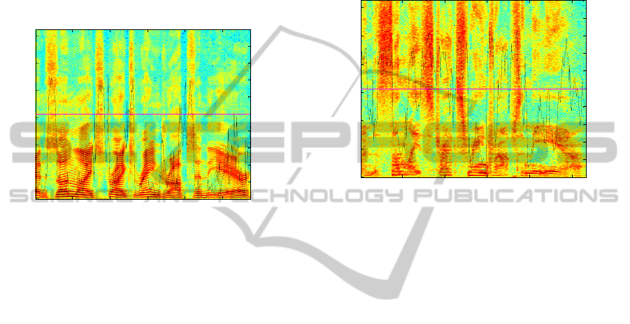
Figure 1: Overlap of the TNI signal on the power spectral

density for the speech signal “RHG1NRL.NSP” (non-

pathological speaker). The horizontal line represents the

threshold used in the turbulence-based decision.

Finally, as high TNI values (in vowels) can be an

indicator of vocal fold pathology, selecting these

frames to detect pathological voices seems to be

more important than using only low TNI ones. This

can be done by specifying a fixed threshold on TNI,

as shown in Figure 1 and Figure 2. All frames with a

TNI value above 0.5 (this value was experimentally

adjusted) are classified as turbulent frames and all

the others are discarded (or taken to another

classifier which uses low turbulent frames).

Figure 1 and Figure 2 contain spectral and TNI

information corresponding to the same excerpts of

the text “The Rainbow Passage” – “When the

sunlight strikes raindrops in the air…”. Although

Figure 1 presents part of an acoustic signal from a

non-pathological male speaker (DVD, 1994), Figure

2 shows the correspondent part of an acoustic signal

from a pathological female speaker. As can be seen,

the fricative sounds (such as /s/), which are

characterized by high energy at higher frequencies,

have low cross-correlation values and,

correspondingly, high TNI values. The voiced

frames, characterized by visible spectral strips, have

higher cross-correlation values, which correspond to

lower TNI values. When comparing the two graphs

it is possible to verify that the fricative sounds in

Figure 2 are considerably more stressed than the

corresponding ones in Figure 1. It is also visible that

some of the voiced parts in Figure 1, characterized

by well-defined formants, are not so well

represented in Figure 2. As an example, in Figure 1

almost all the frames between the 57th and 65th

were classified as non-turbulent (TNI values below

0.5), while in Figure 2, the same frames were

considered as turbulent (TNI values above 0.5).

Figure 2: Overlap of the TNI signal on the power spectral

density for the speech signal “LXC06R.NSP”

(pathological speaker). The horizontal line represents the

threshold used in the turbulence-based decision.

3.4 Classifiers

Since the class information corresponding to each

signal file is available, a supervised learning

classifier, such as a multilayer perceptron (MLP)

neural network, is suitable system. Three MLPs

were trained with the training datasets: one with all

the information (non-turbulent and turbulent

frames); another one with only non-turbulent

information; and the last one using solely turbulent

information. Each MLP was composed of three

layers. Each input consisted of (2N

+ 1) × N

values,

where N

is the number of context frames (for each

frame we considered the influence of the N

preceding frames and the influence of the N

subsequent frames) and N

is the number of

coefficients included in each feature vector (26

coefficients). In the hidden layer 100 hidden neurons

were used. In addition, and due to the reduced

number of frames of the MLP trained with turbulent

information, tests using MLPs with only 25 hidden

neurons were also made. In all cases, each MLP

provided one output. The transfer function for all

units is the sigmoid. The MLPs were initialized

randomly and the training was performed using the

resilient backpropagation algorithm (RPROP).

During training, the weights and biases of the network

umber of frames

Frequency

50 100 150 200 250

2000

4000

6000

8000

10000

12000

0.1

0.2

0.3

0.4

0.5

0.6

0.7

0.8

0.9

TNI

umber of frames

Frequency

50 100 150 200 250

2000

4000

6000

8000

10000

12000

0.1

0.2

0.3

0.4

0.5

0.6

0.7

0.8

0.9

TNI

PATHOLOGICAL VOICE DETECTION USING TURBULENT SPEECH SEGMENTS

241

were iteratively adjusted according to the default

performance function – mean square error (MSE).

4 RESULTS AND DISCUSSION

The objective of this work is to distinguish between

normal and pathological voices, so two classes must

be used. In our case “0” represents the “normal”

class and “1” represents the “pathological” class.

Since there are only two possible decisions, a

statistical hypothesis test can be used. In this

context, the hypothesis H

, or null hypothesis,

indicates that an acoustic sample is pathological and

the hypothesis H

, also referred to as the alternative

hypothesis, means that it is normal. Accepting H

equivalent to rejecting H

and vice versa. When

classifying a sample s, four situations can occur: i)

we make a correct acceptance (CA); ii) we reject the

true hypothesis, which is called wrong rejection

(WR); iii) we make a correct rejection (CR); and iv)

we accept a false hypothesis, which is called wrong

acceptance (WA) also known as false alarm (FA).

The objective of a neural network classifier is to

learn how to characterize each output according to

the information available on the input. In this case,

this means that the classifier should be able to

capture the essence of the “normal” and

“pathological” classes and produce a corresponding

output. Varying the threshold value

, from its

minimum up to its maximum, corresponds to

varying the realizations of the four hypotheses (CA,

WR, CR and WA) and therefore their probabilities:

P(CA|

), P(FR|

), P(CR|

) and P(FA|

). The

realizations of these quantities are achieved as

follows. Given an acoustic signal, the classifier

returns an output for each one of its frames. The

arithmetic mean of the logit values (log(p(1-p)) of

those frames represents a single value, usually called

a score, that characterizes the acoustic signal and

which can be directly compared to the threshold. If

the score is greater than the threshold, then the

acoustic signal is classified as “pathological”.

The optimum threshold value, often referred to

as optimum operation point (OOP), is found

somewhere near where both curves of the histogram

intersect. Another way to find the OOP is to use a

receiver operating characteristic (ROC) curve or a

detection error trade-off (DET) curve (Martin, et al.,

1997). The most widely used OOP consists in

finding the point where WR equals WA and is called

the equal error rate (EER) point. Another way to

define a OOP is to find the point which minimizes

the distance to the origin of the axes in the DET

curve – using the Euclidean distance. All OOPs were

defined in this work using the criterion based on the

Euclidean distance. The results obtained for all

classifiers and for the 4-fold datasets are shown in

Table 2. The figures given represent the sum of all

values (CA, CR, WA, WR) of the four test datasets

specified. The percentage value in the table is

Accuracy which is defined as 100 × (CA+CR)/

(CA+CR+WA+WR).

Table 2: Classifiers’ performance in terms of CA, CR, FA,

FR and accuracy.

Predicted Predicted Tota

All Frames

Pathol. 734 2 736

Normal 2 42 44

Tota

736 44

99.5%

Non-

turbulent

Frames

Pathol. 733 3 736

Normal 3 41 44

Tota

736 44

99.2%

Turbulent

Frames

Pathol. 736 0 736

Normal 0 44 44

Tota

736 44

100%

4.1 Discussion

As shown in Table 2, the worst results were obtained

for the classifier with non-turbulent frames as inputs.

Even in this case, an accuracy of 99.2 ± 0.8% was

achieved, which is 3% better than the results

obtained with the voiced frames based classifier

proposed in (Godino-Llorente, et al.,2009). This

difference can be explained by the context included

in the inputs of the MLPs. Instead of considering

each input as an isolated frame, we use a set of 11

frames each time (5 before, 5 after and the actual

frame). So, the neural network classifiers have more

data to learn from. Another point that can justify the

results obtained is the relation between the selection

of frames and the computation of the first

derivatives of the MFCCs. Since we only select the

frames for the different classifiers after the

computation of the deltas, each frame includes the

influence of its adjacent frames, independently of

the frame type. This means, for example, that the

deltas of a turbulent frame may have been calculated

with the MFCCs of adjacent non-turbulent frames.

More impressive are the results obtained with the

turbulent frame classifier. In all the 4 tests made

with this classifier, a 100% correct classification was

obtained. These results are better than the ones

obtained for the other two classifiers (which are

similar: 99.5 ± 0.9%, for the classifier with all

frames and 99.2 + 0.8%, for the classifier with non-

BIOSIGNALS 2012 - International Conference on Bio-inspired Systems and Signal Processing

242

turbulent frames). Since the algorithm for choosing

frames is based on a TNI implementation and not on

pitch, the frames selected as turbulent contain

important information about the “normality” or the

“pathology” of the speaker. While in the “normal”

cases these frames correspond mostly to fricative

sounds and other unvoiced consonants, in the case of

the pathological speakers the frames also include

vowels with low quality or even whispered (which

does not happen in the case of the classifier with

non-turbulent frames). The classifier with turbulent

frames thus has more relevant data to characterize

and distinguish between both classes and for this

reason it can perform better than the others.

Some tests were also performed in order to

evaluate the influence of the number of context

frames and the number of hidden neurons on the

classifiers’ performance. As expected, the results

proved that the classifiers’ performance decreased as

the number of context frames decreased and/or the

number of hidden neurons also decreased. In

addition to the tests described, some others using

similar MLPs neural networks but with two outputs

instead of one were also performed. The results

obtained were the same as the ones stated before,

which confirms the choice to train classifiers with

only one output.

The results presented this section demonstrate

that the combination of continuous speech along

with turbulent information produces excellent

normal/pathological discrimination results when

using the KayPentax database. However, it does not

imply that the three classifiers succeeded in

obtaining the fundamental cues for “normality” and

“pathology”, independently of the database or the

text. In the literature so far produced it is not

common to see this sort of analysis, which can show

the true meaning of the results obtained.

5 CONCLUSIONS

In this work an algorithm to discriminate normal

from pathological speakers based on the analysis of

turbulent information of continuous speech is

presented. All previous works on this subject assume

that the unvoiced parts of the acoustic signals have

no useful information, which justifies the selection

of only voiced speech segments for their

classification systems. In our opinion, these studies

are in fact disregarding important pathological

information that may appear in unvoiced or almost

unvoiced segments, due to a lower quality of the

vowels produced by speakers with pathologies. To

select the less voiced and unvoiced regions of the

signal we propose a segmentation algorithm based

on an acoustic measure called turbulent noise index,

TNI. By properly adjusting a threshold it is possible

to use the TNI measure to select, among others,

meaningful frames containing vowels with low

quality or even whispered speech. Thus, relevant

pathological information is given to the classifier.

The tests performed in a well-known database

resulted in very good discrimination of the

pathological voices. This result must be emphasized

as it shows that it is possible to correctly classify

normal and pathological speakers according to

turbulent information only.

REFERENCES

Deliyski, D., 1993. Acoustic model and evaluation of

pathological voice production, in: 3rd Conference on

Speech Communication and Technology.

Krom, G., 1993. A cepstrum-based technique for

determining a harmonics-to-noise ratio in speech

signals, J. Speech Hear. Res. 36 (1993) 254-266.

Hillenbrand, J., Houde, R-, 1996. Acoustic correlates of

breathy vocal quality: dysphonic voices and

continuous speech, J. Speech Hear. Res. 39.

Michaelis, D., Gramss, T., 1997. H.W. Strube, Glottal-to-

noise excitation ratio – a new measure for describing

pathological voices, Acta Acustica 83 (1997) 700-706.

Kasuya, H., Ogawa, S., Mashima, K., Ebihara, S, 1986..

Normalized noise energy as an acoustic measure to

evaluate pathologic voice, J. Acoust. Soc. Am. 80 (5)

(1986) 1329-1334.

Klingholtz, F., 1990. Acoustic recognition of voice

disorders: a comparative study of running speech

versus sustained vowels, J. Acoust. Soc. Am. 87.

de Krom, G., 1995. Some spectral correlates of pathological

breathy and rough voice quality for different types of

vowel fragments. J. Speech Hear. Res. 38.

Godino-Llorente, J., Fraile, R., Sáenz-Lechón, N., Osma-

Ruiz, V., Gómez-Vilda, P., 2009. Automatic detection

of voice impairments from text-dependent running

speech, J. Biomed. Signal Process. Control 4.

Mitev, P. ,Hadjitodorov, S., 2000. A method for turbulent

noise estimation in voiced signals, J. Med. Biol. Eng.

Comput., 38, 625-631.

DVD 1994. Massachusetts Eye and Ear Infirmary Voice

and Speech Lab, Disordered Voice Database version

1.03, Kay Elemetrics Corp., Pine Brook, NJ.

Boersma, P., 1993. Accurate short-term analysis of the

fundamental frequency and the harmonics-to-noise

ratio of a sampled sound, Proceedings of the Institute

of Phonetic Sciences 17, 97-110.

Martin, A. et al., 1997. The DET curve in assessment of

detection task performance, in: 5th European

Conference on Speech Communication and

technology – EuroSpeech 1997, 1895-1898.

PATHOLOGICAL VOICE DETECTION USING TURBULENT SPEECH SEGMENTS

243