ESTIMATION OF THE COMMON OSCILLATION

FOR PHASE LOCKED MATRIX FACTORIZATION

Miguel Almeida

1,2

, Ricardo Vig´ario

and Jos´e Bioucas-Dias

Institute of Telecommunications, Instituto Superior T´ecnico, Lisbon, Portugal

Adaptive Informatics Research Centre, Aalto University School of Science, Finland

Keywords:

Matrix factorization, Phase synchrony, Phase-locking, Independent component analysis, Blind source

separation, Convex optimization.

Abstract:

Phase Locked Matrix Factorization (PLMF) is an algorithm to perform separation of synchronous sources.

Such a problem cannot be addressed by orthodox methods such as Independent Component Analysis, because

synchronous sources are highly mutually dependent. PLMF separates available data into the mixing matrix

and the sources; the sources are then decomposed into amplitude and phase components. Previously, PLMF

was applicable only if the oscillatory component, common to all synchronized sources, was known, which

is clearly a restrictive assumption. The main goal of this paper is to present a version of PLMF where this

assumption is no longer needed – the oscillatory component can be estimated alongside all the other variables,

thus making PLMF much more applicable to real-world data. Furthermore, the optimization procedures in

the original PLMF are improved. Results on simulated data illustrate that this new approach successfully

estimates the oscillatory component, together with the remaining variables, showing that the general problem

of separation of synchronous sources can now be tackled.

1 INTRODUCTION

Synchrony is an increasingly studied topic in modern

science. On one hand, there is an elegant yet deep

mathematical framework which is applicable to many

domains where synchrony is present, including laser

interferometry, the gravitational pull of stellar objects,

and the human brain (Pikovsky et al., 2001).

It is believed that synchrony plays an important

role in the way different sections of human brain in-

teract. For example, when humans perform a motor

task, several brain regions oscillate coherently with

the muscle’s electromyogram (EMG) (Palva et al.,

2005; Schoffelen et al., 2008). Also, processes such

as memorization and learning have been associated

with synchrony; several pathologies such as autism,

Alzheimer’s and Parkinson’s are associated with a

disruption in the synchronization proﬁle of the brain;

and epilepsy is associated with an anomalous increase

in synchrony (Uhlhaas and Singer, 2006).

To infer knowledge on the synchrony of the net-

works present in the brain or in other real-world sys-

tems, one must have access to the dynamics of the

individual oscillators (which we will call “sources”).

Usually, in the brain electroencephalogram (EEG)

and magnetoencephalogram (MEG), and other real-

world situations, individual oscillator signals are not

directly measurable; one has only access to a superpo-

sition of the sources.

In fact, EEG and MEG signals

measured in one sensor contain components coming

from severalbrain regions (Nunez et al., 1997). In this

case, spurious synchrony occurs, as has been shown

both empirically and theoretically in previous works

(Almeida et al., 2011a). We brieﬂy review this evi-

dence in Section 2.3.

Undoing this superposition is usually called a

blind source separation (BSS) problem. Typically,

one assumes that the mixing is linear and instanta-

neous, which is a valid and common approximation

in brain signals (Vig´ario et al., 2000) and other ap-

plications. In this case, if the vector of sources is

denoted by s(t) and the vector of measurements by

x(t), they are related through x(t) = Ms(t) where

M is a real matrix called the mixing matrix. Even

with this assumption, the BSS problem is ill-posed:

In EEG and MEG, the sources are not individual neu-

rons, whose oscillations are too weak to be detected from

outside the scalp even with no superposition. In this case,

the sources are populations of closely located neurons os-

cillating together.

Almeida M., Vigário R. and Bioucas-Dias J. (2012).

ESTIMATION OF THE COMMON OSCILLATION FOR PHASE LOCKED MATRIX FACTORIZATION.

In Proceedings of the 1st International Conference on Pattern Recognition Applications and Methods, pages 78-85

DOI: 10.5220/0003774300780085

 SciTePress

there are inﬁnitely many solutions. Thus, one must

also make some assumptions on the sources, such as

statistical independence in Independent Component

Analysis (ICA) (Hyv¨arinen et al., 2001). However,

in the case discussed in this paper, independence of

the sources is not a valid assumption, because syn-

chronous sources are highly dependent. In this paper

we address the problem of how to separate these de-

pendent sources, a problem we name Separation of

Synchronous Sources, or Synchronous Source Sepa-

ration (SSS). Although many possible formal models

for synchrony exist (see, e.g., (Pikovsky et al., 2001)

and references therein), in this paper we use a simple

yet popular measure of synchrony: the Phase Lock-

ing Factor (PLF), or Phase Locking Value (PLV). The

PLF between two signals is 1 if they are perfectly syn-

chronized. Thus, in this paper we tackle the problem

of source separation where all pairs of sources have a

PLF of 1.

A more general problem has also been addressed,

where the sources are organized in subspaces, with

sources in the same subspace having strong syn-

chrony and sources in different subspaces having

weak synchrony. This general problem was tackled

with a two-stage algorithm called Independent Phase

Analysis (IPA) which performed well in the noiseless

case (Almeida et al., 2010) and with moderate lev-

els of added Gaussian white noise (Almeida et al.,

2011a). In short, IPA uses TDSEP (Ziehe and M¨uller,

1998) to separate the subspaces from one another.

Then, each subspace is a separate SSS problem; IPA

uses an optimization procedure to complete the intra-

subspace separation. Although IPA performs well for

the noiseless case, and for various types of sources

and subspace structures, and can even tolerate moder-

ate amounts of noise, its performance for higher noise

levels is unsatisfactory. Also, in its current form, IPA

is limited to square mixing matrices, i.e., to a num-

ber of measurements equal to the number of sources.

It may as well return singular solutions, where two

or more estimated sources are (almost) identical. On

the other hand, IPA can deal with subspaces of phase-

locked sources and with sources that are not perfectly

phase-locked (Almeida et al., 2011a).

In this paper we address an alternative technique,

named Phase Locked Matrix Factorization (PLMF).

PLMF was originally introduced in (Almeida et al.,

2011b), using a very restrictive assumption, of prior

knowledge of the oscillation common to all the

sources. The goal of this paper is to remove this re-

strictive assumption, and to improve the optimization

of the problem.

Unlike IPA, PLMF can deal with higher amounts

of noise and with non-square mixing matrices (more

measurements than sources). Furthermore, it only

uses variables directly related with the data model,

and is immune to singular solutions. PLMF is in-

spired on the well-known Non-negative Matrix Fac-

torization (NMF) approach (Lee and Seung, 2001),

which is not applicable directly to the SSS problem,

because some factors in the factorization are not pos-

itive, as will be made clear below. For simplicity, we

will restrict ourselves to the case where the sources

are perfectly synchronized.

One should not consider PLMF as a replacement

for IPA, but rather as a different approach to a similar

problem: PLMF is a model-drivenalgorithm, whereas

IPA is data-driven. As we will show, PLMF has ad-

vantages and disadvantages relative to IPA.

This paper is organized as follows. In Sec. 2 we

introduce the Phase Locking Factor (PLF) quantity

which measures the degree of synchronization of two

signals, and show that full synchronization between

two signals has a very simple mathematical character-

ization. Sec. 3 describes the PLMF algorithm in de-

tail. In Sec. 4 we explain how the simulated data was

generated and show the results obtained by PLMF. Di-

rections for future work are discussed in Sec. 5. Con-

clusions are drawn in Sec. 6.

2 PHASE SYNCHRONY

2.1 Phase of a Real-valued Signal

In this paper we tackle the problem of Separation

of Synchronous Sources (SSS). The sources are as-

sumed to be synchronous, or phase-locked: thus, one

must be able to extract the phase of a given signal.

In many real-world applications, such as brain EEG

or MEG, the set of measurements available is real-

valued. In those cases, to obtain the phase of such

measurements, it is usually convenient to construct

a set of complex-valued data from them. Two ap-

proaches have been used in the literature: complex

wavelet transforms (Torrence and Compo, 1998) and

the Hilbert transform (Gold et al., 1973).

In this paper we present only results on simulated

data, which is directly generated as complex-valued,

thus curcumventing this issue.

2.2 Phase-locking Factor

Let φ

(t) and φ

(t), for t = 1,..., T, be the time-

dependent phases of signals j and k. The real-valued

“Real-valued” is used here to distinguish from other pa-

pers, where the absolute value operator is dropped, hence

ESTIMATION OF THE COMMON OSCILLATION FOR PHASE LOCKED MATRIX FACTORIZATION

Phase Locking Factor (PLF) between those two sig-

nals is deﬁned as

≡



∑

t=1

[

(t)−φ

(t)

]



(

−φ

)



, (1)

where h·i is the time average operator, and i =

√

−1.

Note that 0 ≤ ρ

≤1. The value ρ

= 1 corresponds

to two signals that are fully synchronized: their phase

lag, deﬁned as φ

(t) −φ

(t), is constant. The value

= 0 is attained if the two phases are not corre-

lated, as long as the observation period T is sufﬁ-

ciently long. Values between 0 and 1 represent par-

tial synchrony. Typically, the PLF values are stored

in a PLF matrix Q such that Q( j, k) ≡ ρ

. Note that

a signal’s PLF with itself is trivially equal to 1: thus,

for all j, ρ

j j

= 1.

2.3 Effect of Mixing on the PLF

The effect of a linear mixing operation on a set of

sources which have all pairwise PLFs equal to 1 is

now discussed. This effect has a simple mathemati-

cal characterization: if s(t) is a set of such sources,

and we deﬁne x(t) ≡ Ms(t), with det(M) 6= 0, then

the only possibility for the observations x to have all

pairwise PLFs equal to 1 is if M is a permutation of

a diagonal matrix (Almeida et al., 2011a). Equiva-

lently, the only possibility for that is if x = s up to

permutation and scaling, a typical non-restrictive in-

determinancy in source separation problems.

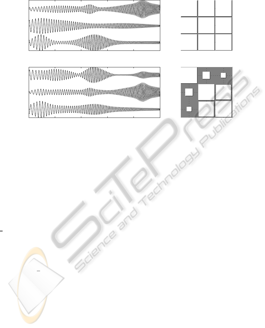
This effect is illustrated in Figure 1, which shows

a set of three perfectly synchronized sources and their

PLFs. That ﬁgure also depicts three signals obtained

througha linear mixing of the sources, and their PLFs.

These mixtures have PLFs lower than 1, in accor-

dance with the result stated in the previous paragraph

(even though the PLF between sources 2 and 3 hap-

pens to be rather high, but still not 1).

This property illustrates that separation of these

sources is necessary to make any type of inference

about their synchrony, as measured through the PLF.

If they are not properly separated, the synchrony val-

ues measured will not be accurate. On the other

hand, established BSS methods such as Independent

Component Analysis (ICA) are not adequate for this

task, since phase-locked sources are not independent

(Almeida et al., 2011a). PLMF is a source separation

algorithm tailored speciﬁcally for this problem, and it

is presented in the next section.

making the PLF a complex quantity (Almeida et al., 2011a).

3 ALGORITHM

We begin with a summary of the notation and deﬁni-

tions used in this section; we then formulate the opti-

mization problem for PLMF and present a table of the

algorithm at the end.

3.1 Assumptions and General

Formulation

We assume that we have a set of N complex-valued

sources s

(t) for j = 1,.. .,N and t = 1,... , T. We

assume also that N is known. Denote by S a N

by T complex-valued matrix whose ( j,t)-th entry is

(t). One can easily separate the amplitude and

phase components of the sources through S = A⊙Φ,

where ⊙ is the elementwise (or Hadamard) product,

A is a real-valued N by T matrix with its ( j,t) ele-

ment deﬁned as a

(t) ≡ |s

(t)|, and Φ is a N by T

complex-valued matrix with its ( j,t) element deﬁned

as Φ

(t) ≡ e

i(angle(s

(t)))

≡ e

iφ

(t)

The representation of S in amplitude and phase is,

thus far, completely general: it merely represents S in

polar coordinates. We place no constraints on A other

than non-negativity, since it its elements are absolute

values of complex numbers. This is consistent with

the use of the PLF as a measure of synchrony: the

PLF uses no information from the signal amplitudes.

We assume that the sources are perfectly synchro-

nized; as discussed in Section 2.2, in this situation,

∆φ

(t) = φ

(t) −φ

(t) is constant for all t, for any j

and k. Thus, Φ can be decomposed as

Φ ≡ zf

, (2)

where z is a complex-valued column vector of size

N containing the relative phase lags of each source,

and f is a complex-valued column vector of size T

containing the common oscillation. In simpler terms,

if the sources are phase-locked, then rank(Φ) = 1,

and the above decomposition is always possible, even

though it is not unique. Then, the time evolution of

each source’s phase is given by φ

(t) = angle(z

) +

angle( f

), where z

and f

are the j-th entry of z and

the t-th element of f, respectively.

Although one can conceive complex-valued

sources where the rows of A and the vector f vary

rapidly with time, in real-world systems we expect

them to vary smoothly; for this reason, as will be seen

below, we chose to softly enforce the smoothness of

these two variables in PLMF.

We also assume that we only have access to P

measurements (P ≥ N) that result from a linear mix-

ing of the sources, as is customary in source separa-

tion problems:

X ≡ MS+ N,

ICPRAM 2012 - International Conference on Pattern Recognition Applications and Methods

1 2 3

0 1000 2000 3000 4000 5000

1 2 3

0 1000 2000 3000 4000 5000

Figure 1: (Top row) Three sources (left) and PLFs between them (right). (Bottom row) Three mixed signals (left) and PLFs

between them (right). On the right column, the area of the square in position (i, j) is proportional to the PLF between the

signals i and j. Therefore, large squares represent PLFs close to 1, while small squares represent values close to zero.

where X is a P by T matrix containing the measure-

ments, M is a P by N real-valued mixing matrix and

N is a P by T complex-valued matrix of noise. Our

assumption of a real mixing matrix is appropriate in

the case of linear and instantaneous mixing, as mo-

tivated earlier. We will deal only with the noiseless

model, where N = 0, although we then also test how

it copes with noisy data.

The goal of PLMF is to recover S and M us-

ing only X. A simple way to do this is to ﬁnd

M and S such that the data misﬁt, deﬁned as



X−M



A⊙(zf

)





, where k·k

is the Frobe-

nius norm, is as small as possible. As mentioned

above, we also want the estimates of A and f to be

smooth. Thus, the minimization problem to be solved

is given by

min

M,A,z,f



X−M



A⊙(zf

)





+ λ

kAD

+ λ

, (3)

s.t.: 1) All elements of M must lie between -1 and +1.

2) All elements of A must be non-negative.

3) All elements of z and f must have

unit absolute value.

where D

and D

are the ﬁrst-order difference oper-

ators of appropriate size, such that the entry ( j,t) of

is given by a

(t) −a

(t + 1), and the k-th en-

try of D

f is given by f

− f

(k+1)

. The ﬁrst term di-

rectly measures the misﬁt between the real data and

the product of the estimated mixing matrix and the es-

timated sources. The second and third terms enforce

smoothness of the rows of A and of the vector f, re-

spectively. These two terms allow for better estimates

for A and f under additive white noise, since enforc-

ing smoothness is likely to ﬁlter the high-frequency

components of that noise.

Constraint 2 ensures that A represents amplitudes,

whereas Constraint 3 ensures that z and f represent

phases. Constraint 1 prevents the mixing matrix M

from exploding to inﬁnity while A goes to zero. Note

that we also penalize indirectly the opposite indeter-

minancy, where M goes to zero while A goes to in-

ﬁnity: that would increase the value of the second

term while keeping the other terms constant, as long

as the rows of A do not haveall elements equal to each

other. Thus, the solution for M lies on the boundary

of the feasible set for M; using this constraint instead

of forcing the L

norm of each row to be exactly 1, as

was done in (Almeida et al., 2011b), makes the sub-

problem for M convex, with all the known advantages

that this brings (Boyd and Vandenberghe, 2004).

3.2 Optimization

The minimization problem presented in Eq. (3) de-

pends on the four variables M, A, z, and f. Although

the minimization problem is not globally convex, it

is convex in A and M individually, while keeping the

other variables ﬁxed. For simplicity, we chose to op-

timize Eq. (3) in each variable at a time, by ﬁrst op-

ESTIMATION OF THE COMMON OSCILLATION FOR PHASE LOCKED MATRIX FACTORIZATION

timizing on M while keeping A, z and f constant;

then doing the same for A, followed by z, and then

f. This cycle is repeated until convergence. From our

experience with the method, the particular order in

which the variables are optimized is not critical. Al-

though this algorithm is not guaranteed to converge

to a global minimum, we have experienced very few

cases of local optima.

In the following, we show that the minimiza-

tion problem above can be translated into well-known

forms (constrained least squares problems) for each

of the four variables. We also detail the optimiza-

tion procedure for each of the four sub-problems. For

brevity, we do not distinguish the real variables such

as M from their estimates

M throughout this section:

in each sub-problem, only one variable is being esti-

mated, while all the others are kept ﬁxed and equal to

their current estimates.

3.2.1 Optimization on M

If we deﬁne m ≡ vec(M) and x ≡ vec(X)

, then the

minimization sub-problem for M, while keeping all

other variables ﬁxed, is equivalent to the following

constrained least-squares problem:

min





R (x)

I (x)



−



R (R)

I (R)





(4)

s.t.: −1 ≤m ≤ +1,

where R (.) and I (.) are the real and imaginary parts,

is the P by P identity matrix, and R ≡ [S

⊗I

with ⊗ denoting the Kronecker product and k·k

de-

noting the Euclidean norm. Here, and throughout

this paper, all inequalities should be understood in the

componentwise sense, i.e., every entry of M is con-

strained to be between -1 and +1. For convenience,

we used the least-squares solver implemented in the

MATLAB Optimization Toolbox to solve this prob-

lem, although many other solvers exist.

The main advantage of using the constraint −1 ≤

M ≤ +1 is now clear: it is very simply translated

into −1 ≤ m ≤ +1 after applying the vec(.) opera-

tor, remaining a convex constraint, whereas other con-

straints would be harder to apply.

3.2.2 Optimization on A

The optimization in A can also be reformulated as a

least-squares problem. If a ≡ vec(A), the minimiza-

tion on A is equivalent to

min







R (x)

I (x)

−N)





−





R (K)

I (K)

√

⊗I







(5)

The vec(.) operator stacks the columns of a matrix into

a column vector.

s.t.: a ≥0,

where K ≡[(Diag(f)⊗M)Diag(z

)], 0

−N)

is a col-

umn vector of size (N

−N), ﬁlled with zeros, and

Diag(.) is a square diagonal matrix of appropriate di-

mension having the input vector on the main diagonal.

We again use the built-in MATLAB solver to solve

this sub-problem.

3.2.3 Optimization on z

The minimization problem in z with no constraints is

equivalent to:

min

kOz−xk

with O =







M Diag(a(1))

M Diag(a(2)))

M Diag(a(T))







(6)

where f

is the t-th entry of f, and a(t) is the t-th col-

umn of A. Usually, the solution of this system will

not obey the unit absolute value constraint. To cir-

cumvent this, we solve this unconstrained linear sys-

tem and afterwards normalize z for all sources j and

time instants t, by transferring its absolute value onto

variable A:

(t) ← |z

(t) and z

← z

/|z

It is easy to see that the new z obtained after this nor-

malization is still a global minimizer of (6) (where the

new value of A should be used).

3.2.4 Optimization on f

Let

x ≡vec(X

). The minimization problem in f with

no constraints can be shown to be equivalent to

min





√



f−



(N−1)





(7)

with P =







∑

Diag(a

)

∑

Diag(a

)

∑

Diag(a

)







where f

is the t-th entry of f, m

is the (i, j) entry of

M, z

is the j-th entry of z, and a

is the j-th row of

As in the sub-problemfor z, in general the solution

of this system will not obey the unit absolute value

constraint. Thus, we perform a similar normalization,

given by

(t) ← |f

(t) and f

← f

/|f

|. (8)

Note that unlike the previous case of the optimization

for z, this normalization changes the cost function, in

ICPRAM 2012 - International Conference on Pattern Recognition Applications and Methods

particular the term λ

. Therefore, there is no

guarantee that after this normalization we have found

a global minimum for f.

For this reason, we construct a vector of angles

β ≡ angle(f) and minimize the cost function (3) as

a function of β, using 20 iterations of Newton’s al-

gorithm. Although inﬁnitely many values of β cor-

respond to a given f, any of those values is suitable.

The advantage of using this new variable is that there

are no constraints in β, so the Newton algorithm can

be used freely. Thus, the normalized solution of the

linear system in (7) can be considered simply as an

initialization for the Newton algorithm on β, which in

most conditions can ﬁnd a local minimum.

On the ﬁrst time that the Newton algorithm is run,

it is initialized using the unconstrained problem (7)

and the ensuing normalization (8). On the second and

following times that it is run, the result of the previous

minimization on f is used as initial value.

3.2.5 Phase Locked Matrix Factorization

The consecutive cycling of optimizations on M, A, z

and f constitutes the Phase Locked Matrix Factoriza-

tion (PLMF) algorithm. A summary of this algorithm

is presented below.

PHASE LOCKED MATRIX FACTORIZATION

1: Input data X

2: Input random initializations

3: for iter ∈ {1,2,...,MaxIter}, do

4: Solve the constrained problem in Eq. (4)

5: Solve the constrained problem in Eq. (5)

6: Solve the unconstrained system in Eq. (6)

7: a

(t) ← |z

(t) and z

← z

/|z

|, j = 1, ... ,N

8: if iter = 1

9: Solve the unconstrained system in Eq. (7)

10: a

(t) ← |f

(t) and f

← f

/|f

|, t = 1, ... ,T

11: Optimize β ≡angle(f) with Newton algorithm

(use result of step 10 as initialization)

12: else

13: Optimize β ≡angle(f) with Newton algorithm

(use Newton algorithm from (iter-1) as init.)

14: end for

4 SIMULATION AND RESULTS

In this section we show results on small simulated

datasets, demonstrating that PLMF can correctly fac-

tor the data X into a mixing matrix M, amplitudes

A, and phases z and f. Despite deriving PLMF for

the noiseless case, we will also test its robustness to a

small noisy perturbation.

4.1 Data Generation

We generate the data directly from the model X =

MS, with S = A⊙Φ = A⊙(zf

), taking N = 2 and

P = 4. The number of time samples is T = 100. M

is taken as a random matrix with entries uniformly

distributed between -1 and +1. We then normalize

M so that the entry with the largest absolute value is

±1. Each row of A (i.e. each source’s amplitude) is

generated as a sum of a constant baseline and 2 to 5

Gaussians with random mean and random variance.

z is generated by uniformly spacing the N sources in

the interval



2π



f is generated as a complex si-

nusoid with angular frequency 0.06 in the ﬁrst half

of the observation period, and angular frequency 0.04

in its second half, in a way that f has no discontinu-

ities. X is then generated according to the data model:

X = M(A⊙(zf

)).

The initial values for the estimated variables are

all random: elements of

M and

A are drawn from the

Uniform([0,1]) distribution (

M is then normalized in

the same way as M), while the elements of

z are of

the form e

iα

with α taken from the Uniform





distribution. The elements of f are also of the form

iβ

, with β uniformly distributed between 0 and 2π.

We generate 100 datasets of each of two types of

datasets with the following features:

• Dataset 1: 2 sources, 4 sensors, 100 time points,

no noise.

• Dataset 2: exactly the same data as dataset 1, plus

complex Gaussian noise with standard deviation

0.1, added after the mixture (additive noise).

4.2 Quality Measures

M can be compared with M through the gain matrix

G ≡

M, where

is the Moore-Penrose pseudo-

inverse of

M (Ben-Israel and Greville, 2003). This is

the same as

−1

M if the number of sensors is equal

to the number of sources. If the estimation is well

done, the gain matrix should be close to a permutation

of the identity matrix. After manually compensating

a possible permutation of the estimated sources, we

compare the sum of the squares of the diagonal el-

ements of G with the sum of the squares of its off-

diagonal elements. This is a criterion not unlike the

well-known Signal-to-Interference Ratio (SIR), but

our criterion depends only on the true and estimated

mixing matrices. Since this criterion is inspired on the

SIR, we call this criterion pseudo-SIR, or pSIR.

This choice of z is done to ensure that the sources never

have phase lags close to 0 or π, which violate the mild as-

sumptions mentioned in Section 2.3 (Almeida et al., 2011a).

ESTIMATION OF THE COMMON OSCILLATION FOR PHASE LOCKED MATRIX FACTORIZATION

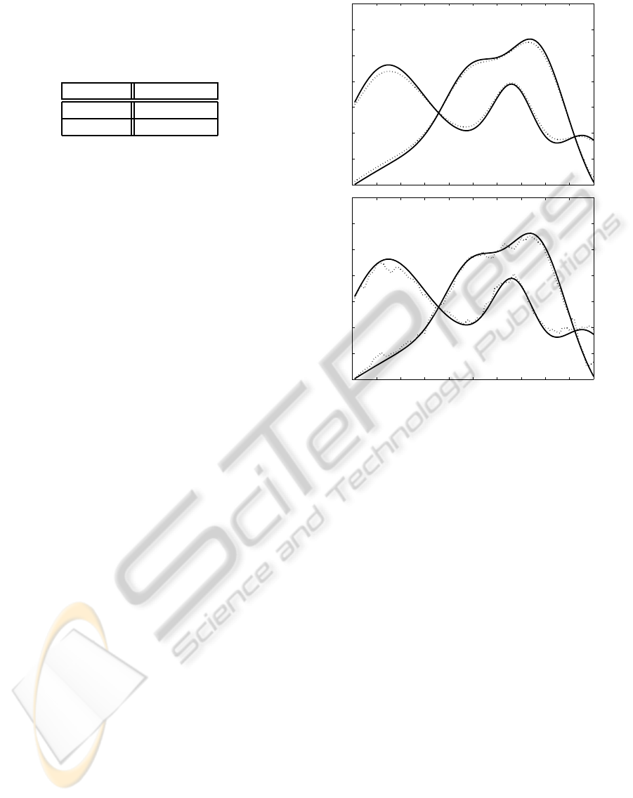
Table 1: Comparison of the estimated mixing matrix

with the true mixing matrix M through the pseudo-SIR of

the gain matrix G ≡

M. For zero noise (dataset 1), the

estimation is quite good, and the performance hit due to the

presence of noise (dataset 2) is minimal.

Data pSIR (dB)

Dataset 1 21.2 ± 11.3

Dataset 2 20.7 ± 11.7

Also,

A will be compared to A through visual in-

spection for one dataset with a pSIR close to the aver-

age pSIR of the 100 datasets.

4.3 Results

We did not implement a convergence criterion; we

simply do 400 cycles of the optimization on M, A, z

and f using λ

= 3 and λ

= 1. The mean and standard

deviation of the pSIR criterion are presented in Ta-

ble 1. Figure 2 shows the results of the estimation of

the source amplitudes for one representative dataset,

showing that

A is quite close to the real A for both the

noiseless and the noisy datasets. Note that if noise is

present, it is impossible to recreate the original ampli-

tudes as they are only present in the data corrupted by

noise: one can thus only estimate the corrupted am-

plitudes. If desired, a simple low-pass ﬁltering proce-

dure can closely recreate the original amplitudes.

These results illustrate that PLMF can separate

phase-locked sources in both the noiseless and the

noisy condition. Furthermore, they show that the per-

formance hit due to the presence of a small amount

of noise is minimal, suggesting that PLMF has good

robustness against small perturbations.

5 DISCUSSION

The above results show that this approach has a

high potential, although some limitations must be ad-

dressed to turn this algorithm practical for real-world

applications.

The values of the parameters that we chose were

somewhat ad hoc. Nevertheless, it is likely that

knowledge of the covariance of the additive noise al-

lows one to choose the values of these parameters op-

timally.

One incomplete aspect of PLMF is its lack of a

stopping criterion; in fact, the results shown in Table

1 could be considerably improved if the number of it-

erations is increased to, say, 1000, although that is not

the case for all of the 100 datasets. We did not tackle

this aspect due to lack of time; however, the data mis-

0 10 20 30 40 50 60 70 80 90 100

0.4

0.6

0.8

1.2

1.4

1.6

1.8

0 10 20 30 40 50 60 70 80 90 100

0.4

0.6

0.8

1.2

1.4

1.6

1.8

Figure 2: Visual comparison of the estimated amplitudes

(dashed lines) with the true amplitudes A (solid lines), for

a representative dataset, after both are normalized so that

they have unit means over the observation period. (Top) Re-

sults for dataset 1: the two estimated amplitudes are close

to the true values. (Bottom) Results for dataset 2: due to

the presence of noise, it is impossible for the two estimated

amplitudes to coincide perfectly with the true ones, but nev-

ertheless the estimated amplitudes follow the real ones very

closely.

ﬁt (ﬁrst term of the cost function) can probably be

used to design a decent criterion.

If the sources are not perfectly phase-locked, their

pairwise phase differences ∆φ

are not constant in

time and therefore one cannot represent the source

phases by a single vector of phase lags z and a single

vector f with a common oscillation. In other words, Φ

will have a rank higher than 1 (in most cases, it will

have the maximum possible rank, which is N), which

makes a representation Φ = zf

impossible. We are

investigating a way to estimate the “most common”

phase oscillation f from the data X, after which PLMF

can be used to initialize a more general algorithm that

estimates the full Φ. We are currently testing also

a more general algorithm, which optimizes Φ with a

gradient descent algorithm. Yet, it is somewhat prone

to local minima, as one would expect for optimizing

variables of size NT = 200. A good initialization is

likely to alleviate this problem.

Another limitation of PLMF is the indetermina-

ICPRAM 2012 - International Conference on Pattern Recognition Applications and Methods

tion that arises if two sources have ∆φ

= 0 or π. In

that case, the problem becomes ill-posed, as was al-

ready the case in IPA (Almeida et al., 2011a). In fact,

using sources with ∆φ

starts to deteriorate the

results of PLMF, even with zero noise.

One further aspect which warrants discussion is

PLMF’s identiﬁability. If we ﬁnd two factorizations

such that X = M



⊙(z

)



= M



⊙(z

)



(i.e., two factorizations which perfectly describe the

same data X), does that imply that M

= M

, and

similar equalities for the other variables? It is quite

clear that the answer is negative: the usual indeter-

minancies of BSS apply to PLMF as well, namely

the indeterminancies of permutation, scaling, and sign

of the estimated sources. There is at least one fur-

ther indeterminancy: starting from a given solution

X = M



⊙(z

)



, one can always construct a

new one by deﬁning z

≡ e

iψ

and f

≡ e

−iψ

while keeping M

≡ M

and A

≡ A

. Note that

= A

⊙(z

) = A

⊙(z

) = S

, thus the esti-

mated sources are exactly the same.

6 CONCLUSIONS

We presented an improved version of Phase Locked

Matrix Factorization (PLMF), an algorithm that di-

rectly tries to reconstruct a set of measured signals as

a linear mixing of phase-locked sources, by factoriz-

ing the data into a product of four variables: the mix-

ing matrix, the source amplitudes, their phase lags,

and a common oscillation.

PLMF is now able to estimate the sources even

when their common oscillation is unknown – an ad-

vantage which greatly increases the applicability of

the algorithm. Furthermore, the sub-problem for M

is now convex, and the sub-problems for z and f are

tackled in a more appropriate manner which should

ﬁnd local minima. The results show good perfor-

mance for the noiseless case and good robustness to

small amounts of noise. The results show as well that

the proposed algorithm is accurate and can deal with

low amounts of noise, under the assumption that the

sources are fully phase-locked, even if the common

oscillation is unknown. This generalization brings us

considerably closer to being able to solve the Separa-

tion of Synchronous Sources (SSS) problem in real-

world data.

ACKNOWLEDGEMENTS

This work was partially funded by the DECA-Bio

project of the Institute of Telecommunications, and

by the Academy of Finland through its Centres of Ex-

cellence Program 2006-2011.

REFERENCES

Almeida, M., Bioucas-Dias, J., and Vig´ario, R. (2010). In-

dependent phase analysis: Separating phase-locked

subspaces. In Proceedings of the Latent Variable

Analysis Conference.

Almeida, M., Schleimer, J.-H., Bioucas-Dias, J., and

Vig´ario, R. (2011a). Source separation and cluster-

ing of phase-locked subspaces. IEEE Transactions on

Neural Networks, 22(9):1419–1434.

Almeida, M., Vigario, R., and Bioucas-Dias, J. (2011b).

Phase locked matrix factorization. In Proc. of the EU-

SIPCO conference.

Ben-Israel, A. and Greville, T. (2003). Generalized in-

verses: theory and applications. Springer-Verlag.

Boyd, S. and Vandenberghe, L. (2004). Convex Optimiza-

tion. Cambridge University Press.

Gold, B., Oppenheim, A. V., and Rader, C. M. (1973). The-

ory and implementation of the discrete hilbert trans-

form. Discrete Signal Processing.

Hyv¨arinen, A., Karhunen, J., and Oja, E. (2001). Indepen-

dent Component Analysis. John Wiley & Sons.

Lee, D. and Seung, H. (2001). Algorithms for non-negative

matrix factorization. In Advances in Neural Informa-

tion Processing Systems, volume 13, pages 556–562.

Nunez, P. L., Srinivasan, R., Westdorp, A. F., Wijesinghe,

R. S., Tucker, D. M., Silberstein, R. B., and Cadusch,

P. J. (1997). EEG coherency I: statistics, refer-

ence electrode, volume conduction, laplacians, cor-

tical imaging, and interpretation at multiple scales.

Electroencephalography and clinical Neurophysiol-

ogy, 103:499–515.

Palva, J. M., Palva, S., and Kaila, K. (2005). Phase syn-

chrony among neuronal oscillations in the human cor-

tex. Journal of Neuroscience, 25(15):3962–3972.

Pikovsky, A., Rosenblum, M., and Kurths, J. (2001). Syn-

chronization: A universal concept in nonlinear sci-

ences. Cambridge Nonlinear Science Series. Cam-

bridge University Press.

Schoffelen, J.-M., Oostenveld, R., and Fries, P. (2008).

Imaging the human motor system’s beta-band syn-

chronization during isometric contraction. NeuroIm-

age, 41:437–447.

Torrence, C. and Compo, G. P. (1998). A practical guide

to wavelet analysis. Bull. of the Am. Meteorological

Society, 79:61–78.

Uhlhaas, P. J. and Singer, W. (2006). Neural synchrony in

brain disorders: Relevance for cognitive dysfunctions

and pathophysiology. Neuron, 52:155–168.

Vig´ario, R., S¨arel¨a, J., Jousm¨aki, V., H¨am¨al¨ainen, M., and

Oja, E. (2000). Independent component approach to

the analysis of EEG and MEG recordings. IEEE

Trans. On Biom. Eng., 47(5):589–593.

Ziehe, A. and M¨uller, K.-R. (1998). TDSEP - an efﬁ-

cient algorithm for blind separation using time struc-

ture. In International Conference on Artiﬁcial Neural

Networks, pages 675–680.

ESTIMATION OF THE COMMON OSCILLATION FOR PHASE LOCKED MATRIX FACTORIZATION