
TERMINATION OF SIMULATED ANNEALING ALGORITHM
SOLVING SEMI-SUPERVISED LINEAR SVMS PROBLEMS
Vaida Bartkute-Norkuniene
Vilnius University, Institute of Informatics and Mathematics, Vilnius, Lithuania
Utena University of Applied Sciences, Utena, Lithuania
Keywords: Order Statistics, Continuous Optimization, Simulated Annealing, Semi-supervised SVMs Classification.
Abstract: In creating heuristic search algorithms one has to deal with the practical problem of terminating and
optimality testing. To solve these problems, we can use information gained from the set of the best function
values (order statistics) provided during optimization. In this paper, we consider the application of order
statistics to establish the optimality in heuristic optimization algorithms and to stop the Simulated Annealing
algorithm when the confidence interval of the minimum becomes less than admissible value. The accuracy
of the solution achieved during optimization and the termination criterion of the algorithm are introduced in
a statistical way. We build a method for the estimation of confidence intervals of the minimum using order
statistics, which is implemented for optimality testing and terminating in Simulated Annealing algorithm. A
termination criterion - length of the confidence interval of the extreme value of the objective function - is
introduced. The efficiency of this approach is discussed using the results of computer modelling. One test
function and two semi-supervised SVMs linear classification problems illustrate the applicability of the
method proposed.
1 INTRODUCTION
The termination problem is topical in stochastic and
heuristic optimization algorithms. Note, values of
the objective function provided during optimization
contain important information on the optimum of the
function and, thus, might be applied to algorithm
termination. Mockus (Mockus, 1967), Zilinskas and
Zhigljavsky (Zilinskas & Zhigljavsky, 1991) were
the first who proposed statistical inferences for
optimality testing in optimization algorithms using
theory of order statistics. These inferences were
studied by computer simulation (see, Bartkute et al,
2005, Bartkute & Sakalauskas, 2009), which
confirmed theoretical assumption about the
distribution of order statistics with respect to
extreme value distribution. Thus, the estimate of
extremum value of the objective function and its
confidence interval were proposed following to
latter assumption. Besides, in Bartkute &
Sakalauskas (Bartkute & Sakalauskas, 2009a) it was
proposed to terminate the stochastic optimization
algorithm, when the confidence interval of the
extremum
becomes less than prescribed value. Since
theoretical analysis of the optimal decision
making
algorithm is complicated, computer modelling
becomes an important research method that enable
us to test and study hypotheses arising from the
problem discussed above. Semi-supervised SVMs
linear classification problems as an examples
illustrate the applicability of the method proposed.
2 METHOD FOR TESTING THE
OPTIMALITY
Assume, the optimization problem is (minimization)
(
)
min→xf
(1)
where
ℜ→ℜ
n
f : is a function bounded from
below,
()
−∞>=
⎟
⎠
⎞
⎜
⎝
⎛
=
ℜ∈
Axfxf
n
x
*
min
, ∞<
*
x . Let
this problem be solved by the Markov type
algorithm providing a sample
{}
N
, ... ,
1
η
η
=Η ,
whose elements are function values
)(
k
xf
k
=
η
.
Our approach is grounded by the assumption on the
asymptotic distribution of order statistics according
to the Weibull (Weibull, 1951) distribution
150
Bartkute-Norkuniene V..
TERMINATION OF SIMULATED ANNEALING ALGORITHM SOLVING SEMI-SUPERVISED LINEAR SVMS PROBLEMS.
DOI: 10.5220/0003759301500156
In Proceedings of the 1st International Conference on Operations Research and Enterprise Systems (ICORES-2012), pages 150-156
ISBN: 978-989-8425-97-3
Copyright
c
2012 SCITEPRESS (Science and Technology Publications, Lda.)

()
()
,0,,0,1,,, >≥>−=
−⋅−
cAxeAcxW
Axc
αα
α
where
c, A and α denote the scale, location and
shape parameters, respectively (see for details
Bartkute & Sakalauskas, 2009a). The Weibull
distribution is one of the extreme-value distributions
which is applied also in optimality testing of Markov
type optimization algorithms. Although this limit
distribution of extreme values is studied mostly for
i.i.d. values, it also might be often used in the
absence of the assumption of independence
(Galambosh, 1984).
To estimate confidence intervals for the
minimum
A of the objective function, it suffices to
choose from sample H only
k+1 the best function
values
NkN ,
, ... ,
,0
η
η
, from the ordered
sample
NNNkNN ,
...
,
,...,
,1,0
η
η
η
η
≤≤≤≤≤ ,
where
()
Nkk = , +∞→→ N,
N
k
0
2
(Zilinskas &
Zhigljavsky, 1991, Bartkute & Sakalauskas, 2009a).
Then the linear estimators for A can be as follows:
()
⎟
⎠
⎞
⎜
⎝
⎛
−⋅−=
0
,,0
,
ηηη
Nk
k
c
N
kN
A
(2)
where coefficient
k
c
can be estimated as
⎟
⎟
⎠
⎞
⎜
⎜
⎝
⎛
−
⎟
⎠
⎞
⎜
⎝
⎛
⋅
+=
∏
=
1
1
11
1
k
i
k
i
c
α
,
α
is the shape parameter of
distribution of the extreme values,
β
α
n
=
,
β
is the
parameter of homogeneity of the function
(
)
xf in
the neighbourhood of the point of
minimum:
()
⎟
⎟
⎠
⎞
⎜
⎜
⎝
⎛
−=
⎟
⎠
⎞
⎜
⎝
⎛
−
β
**
xxOxfxf
(Zilinskas &
Zhigljavsky, 1991, Bartkute & Sakalauskas, 2009a).
The one-side confidence interval of the
minimum of the objective function is as follows:
[
NNNk
k
r
N ,0
,
,0,
,
,0
ηηη
γ
η
⎟
⎠
⎞
⎜
⎝
⎛
−⋅−
]
(3)
where
() ()
⎟
⎟
⎟
⎟
⎟
⎟
⎠
⎞
⎜
⎜
⎜
⎜
⎜
⎜
⎝
⎛
⎟
⎟
⎟
⎟
⎠
⎞
⎜
⎜
⎜
⎜
⎝
⎛
−−−
⎟
⎟
⎟
⎟
⎠
⎞
⎜
⎜
⎜
⎜
⎝
⎛
−−=
αα
γ
δδ
1
1
1
1
,
11111
kk
k
r
,
γ
is
the confidence level.
The estimates introduced here might be used to
create the termination criterion for the stochastic and
heuristic optimization algorithms, namely, the
algorithm stops, when the length of the confidence
interval becomes less than prescribed value
0>
ε
.
3 DESCRIPTION OF SIMULATED
ANNEALING ALGORITHM
Let us consider an application of this approach to
continuous global optimization by the Simulated
Annealing algorithm (SA). This is a well-known
Markov type algorithm for random optimization.
Simulated Annealing (SA) is widely applied in
multiextremal problems. Conditions of global
convergence of SA are studied by many authors
(Granville et al., 1994, Yang, 2000, etc.). We use the
modification of SA, developed by Yang (2000),
where the function regulating the neighbourhood
depth of solution is introduced together with the
temperature regulation function. The procedure of
the SA algorithm consists of the following steps:
Step 1. Choose an initial point
n
Dx ℜ⊂∈
0
, an
initial temperature value
0
0
>T
, a kind of
temperature-dependent generation probability
density function, a corresponding temperature
updating function, and a sequence
}0,{ ≥t
t
ρ
of
monotonically decreasing positive numbers,
describing the neighboring states. Calculate
)(
0
xf
.
Set
0
=
t .
Step 2. Generate a random vector
t
z by using
the generation probability density function. If there
exists i such that
t
t
i
z
ρ
<
,
ni ≤≤1
, where
t
i
z
is the
i
th
component of the vector
t
z
, repeat Step 2.
Otherwise, generate a new trial point
t
y
by adding
the random vector
t
z
to the current iteration point
t
x
,
ttt
zxy +=
(4)
If
Dy
t
∉ , repeat Step 2; otherwise, calculate
)(
t
yf .
Step 3. Use the Metropolis acceptance criterion
to determine a new iteration point
1+t
x
[10].
Specifically, generate a random number
κ
with the
uniform distribution over [0,1], and then calculate
the probability
(
)
t
tt
TxyP ,,
of accepting the trial
point
t
y as the new itteration point
1+t
x
, given
t
x and
t
T ,
⎪
⎭
⎪
⎬
⎫
⎪
⎩
⎪
⎨
⎧
⎟
⎟
⎠
⎞
⎜
⎜
⎝
⎛
−
=
t
tt
t
tt
T
yfxf
TxyP
)()(
exp,1min),,(
.
TERMINATION OF SIMULATED ANNEALING ALGORITHM SOLVING SEMI-SUPERVISED LINEAR SVMS
PROBLEMS
151

If
(
)
t
tt
TxyP ,,≤
κ
, set
tt
yx =
+1
and
(
)
(
)
tt
yfxf =
+1
; otherwise, set
tt
xx =
+1
and
(
)
(
)
tt
xfxf =
+1
.
Step 4.
If the prescribed termination condition is
satisfied, then stop; otherwise, update the value of
the temperature by means of the temperature
updating function, and then go back to Step 2.
Thus, by applying the generation mechanism and
the Metropolis acceptance criterion, the SA
algorithm produces two sequences of random points.
These are the sequence
{
}
0, ≥ty
t
of trial points
generated by (4) and the sequence
{
}
0, ≥tx
t
of
iteration points determined by applying the
Metropolis acceptance criterion as described in Step
3. These two sequences of random variables are all
dependent on the temperature sequence
{
}
0, ≥tT
t
determined by the temperature updating function,
the state neighbouring sequence
{}
0, ≥t
t
ρ
, and the
approach of random vector generation.
The sequence
{}
0, ≥t
t
ρ
of positive numbers
specified in Step 1 of the above SA algorithm is
used to impose a lower bound on the random vector,
generated at the each iteration, for obtaining the
random trial point. This lower bound should be
small enough and monotonically decreasing as the
annealing proceeds. Since the temperature-
dependent generation probability density function is
used to generate random trial points and since only
one trial point is generated at each temperature value
the SA algorithm considered is characterized by a
nonhomogeneous continuous-state Markov chain.
The convergence conditions of the SA were
studied by Yang (Yang, 2000) and several updating
functions for the method parameters were given,
which ensure convergence of the method. We
applied the next updating functions in testing our
approach.
Let
n
r ℜ∈
, with component
ii
Dyx
i
yxr −=
∈,
max
,
ni ≤≤1
,
1>d
,
1>u
,
u
<
<
λ
0
,
i
ni
r
≤≤
<<
1
0
min0
ρ
,
nu
t
t
⋅
−
⋅=
λ
ρρ
0
for all
1≥t
, where
{}
0, ≥t
t
ρ
is the sequence used to impose lower
bounds on the random vectors generated in the SA
algorithm. Let the temperature-dependent generation
probability density function
()
t
Tp ,⋅
be given by
.,1log1
2
)1(
),(
1
n
d
t
i
n
i
t
i
t
t
z
T
z
T
z
T
a
Tzp ℜ∈
⎟
⎟
⎠
⎞
⎜
⎜
⎝
⎛
⎟
⎟
⎠
⎞
⎜
⎜
⎝
⎛
+
⎟
⎟
⎠
⎞
⎜
⎜
⎝
⎛
+⋅
−
=
∏
=
Then, for any initial point
Dx ∈
0
, the sequence
{
}
0);( ≥txf
t
of objective function values converges
in probability to the global minimum
*
f
, if the
temperature sequence
{
}
0, ≥tT
t
determined by the
temperature updating function satisfies the following
condition:
⎟
⎟
⎟
⎠
⎞
⎜
⎜
⎜
⎝
⎛
⋅−⋅=
⋅nd
t
tlTT
1
0
exp
,
...,,,i 21=
where
0
0
>T
is the initial temperature value and
0>l
is a given real number (Yang, 2000).
Typically a different form of the temperature
updating function has to be used with respect to a
different kind of the generation probability density
function in order to ensure the global convergence of
the corresponding SA algorithm. Furthermore, the
flatter is the tail of the generation probability
function, the faster is the decrement of the
temperature sequence determined by the temperature
updating function.
4 SVM CLASSIFICATION
Data classification is a common problem in science
and engineering. Support Vector Machines (SVMs)
are powerful tools for classifying data that are often
used in data mining operations.
In the standard binary classification problem, a
set of training data
(
)
ii
y,u , … ,
(
)
mm
y,u is
observed, where the input set of points is
ni
Uu ℜ⊂∈ , the
i
y is either +1 or −1, indicating
the class to which the point
i
u belongs,
{
}
11 −+∈ ,y
i
. The learning task is to create the
classification rule
{}
11 −+→ ,U:f that will be
used to predict the labels for new inputs. The basic
idea of SVMs classification is to find a maximal
margin separating hyperplane between two classes.
It was first described by Cortes and Vapnik (Cortes
& Vapnik, 1995). The standard binary SVM
classification problem is shown visually in Figure 1.
ICORES 2012 - 1st International Conference on Operations Research and Enterprise Systems
152

Figure 1: Linear separating hyperplanes for a separable
case.
4.1 Semi-supervised Linear SVMs
There are a lot of classification problems where data
labeling is hard or expensive, while unlabeled data is
often abundant and cheap to collect. The typical
areas where this happens is the speech processing,
text categorization, webpage classification, business
risk identification, credit scoring and, finally, a
bioinformatics area where it is usually both
expensive and slow to label huge number of data
produced. When data points consist of exactly two
sets: one set that has been labeled by a decision
maker and the other that is not classified, but
belongs to one known category we have a traditional
semi-supervised classification problem (Bennett &
Demiriz (1999), Huang & Kecman (2004)). The goal
of semi-supervised classification is to use unlabeled
data to improve the performance of standard
supervised learning algorithms. In semi-supervised
learning the data set
{
}
n
i
i
uU
1=
=
can be divided into
two parts: the training set consists of
p labelled
examples
(){}
p
i
ii
y,u
1=
,
1±=
i
y
, and of m unlabeled
examples
{}
n
pi
i
u
1+=
, with m
p
n += . The learning
task is to create the classification rule
{}
11 −+→ ,U:f
that will be used to predict the
labels for new inputs. To solve that problem we may
rewrite standard binary classification problem
(Cortes & Vapnik, 1995) in the following
unconstrained form (Astorino & Fuduli, 2007,
Bartkute-Norkuniene, 2009b):
()
bwf
b
n
w
,min
, ℜ∈ℜ∈
,
where
()
()()
++⋅⋅⋅+=
∑
=
p
i
iTi
buwyLC
w
bwf
1
1
2
2
,
∑
+
+=
⎟
⎠
⎞
⎜
⎝
⎛
+⋅⋅+
pm
pi
iT
buwLC
1
2
w
and b are both the hyperplane parameters,
(
)
(
)
t,maxtL
−
=
10
,
(
) ()
t,maxtL −= 10
are the loss
functions,
0
21
≥≥ CC
are certain penalty
coefficients,
p is the size of training set, and m is the
size of testing set. The first two terms in the
objective function
(
)
b,wf
define the standard SVM,
and the third one incorporates unlabelled (testing)
data. The error over labelled and unlabelled
examples is weighted by two parameters
C
1
and C
2
.
This form seems advantageous especially when the
input dataset is very large.
5 COMPUTER MODELLING
The empirical evidence of our approach, using two
test functions, synthetic and real datasets, is
provided and discussed in this Section. To evaluate
the performance of our proposed algorithm in
practice, we analyze two machine learning datasets.
Example 1: test function (Zhigljavsky &
Zilinskas, 2007)
()
()
()()
()()
()()
()
⎪
⎪
⎪
⎪
⎩
⎪
⎪
⎪
⎪
⎨
⎧
⎥
⎦
⎤
⎢
⎣
⎡
−
∈−
⎥
⎦
⎤
⎢
⎣
⎡
−−−
∈
⎟
⎠
⎞
⎜
⎝
⎛
−
−
⎥
⎦
⎤
⎢
⎣
⎡
−−
∈
⎟
⎟
⎠
⎞
⎜
⎜
⎝
⎛
−−
−
=
1,
1
sin
2
1
1
1
,
11
1
sin1
11
,0
11
sin
2
1
1
2
2
2
,
l
l
xforxl
l
l
sl
ls
xfor
l
xls
sl
ls
xfor
ls
xls
xf
ls
π
π
π
For all integer
2, ≥ls
, the functions
()
(
)
xf
ls,
are continuously differentiable in the set
[]
1,0
and
have three local minima. These local minima are
achieved at the points:
(
)
(
)
(
)( )
l
x
sl
ls
x
sl
ls
x
2
1
1,
2
112
,
2
11
321
−=
−−
=
−
−
=
.
Global minimum is at the point
2
x
and equal to
0. Despite the fact that the functions
()
(
)
xf
ls,
are
continuously differentiable, the problem of finding
the minimum point is very difficult when
k is large.
Example 2: The Rastrigin function
() ( )
(
)
∑
=
⋅−+=
n
i
ii
xxnxf
1
2
2cos1010
π
, search domain
is
2,12.512.5 =≤≤− nx
i
, the minimum is 0.
TERMINATION OF SIMULATED ANNEALING ALGORITHM SOLVING SEMI-SUPERVISED LINEAR SVMS
PROBLEMS
153
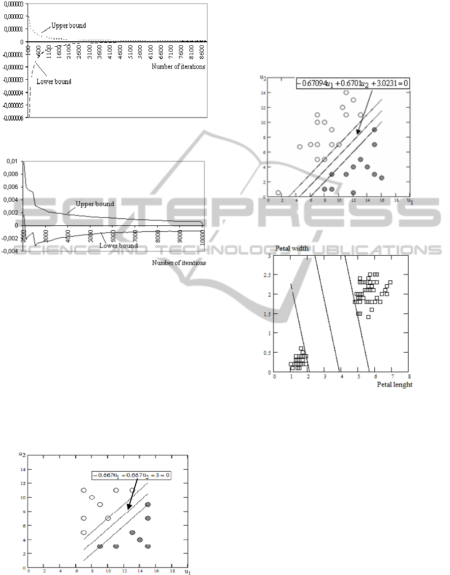
Figure 2: Confidence bounds of the minimum (Example 1,
s=12, l=5).
Figure 3: Confidence bounds of the minimum (Example
2).
Test functions were minimized, with the number
of iterations
N =10000 and the number of trials
M=500, starting from points randomly distributed in
the search domain. Results of the estimate (2) of the
test functions minimum value
kN
A
,
and the estimate
(3) of the confidence interval are presented in Table
1 and Figures 2 and 3. These results show that the
proposed estimates approximate the confidence
interval of the objective function minimum value
rather well, and that the length of the confidence
interval decreases when the number of iterations
increases.
Figure 4: Linear separating hyperplanes of training data.
Example 3: linear example (V. Bartkute-
Norkuniene (2009). The linear separating
hyperplanes of training data are demonstrated in
Figure 4. Figure 5 illustrates that the SA classifier
for training and testing datasets is close to an
optimal decision boundary.
Figure 5: Linear separating hyperplanes of the training and
testing data.
Figure 6: Linear separating hyperplanes for two
dimensional Iris Plant data,
b= 2.1830, w
1
=-0.5625,
w
2
= -0.2741.
Example 4: dataset of Iris Plants (Asuncion &
Newman, 2007). The dataset contains 3 classes of 50
instances each, where each class refers to a type of
iris plant. One class is linearly separable from the
other two, the latter are not linearly separable from
each other. In our approach for the binary
classification we use only two classes of iris plant:
iris Setosa (the class +1) and iris Virginica (the class
-1).
Linear separating hyperplanes for two-
dimensional Iris Plant data are illustrated in Figure
6. These results illustrate the applicability of SA
algorithm for Semi-supervised SVM classification.
In Figure 7,
we can see histograms of the number
of iterations after termination of the SA algorithm
depending on the length of the confidence interval.
ICORES 2012 - 1st International Conference on Operations Research and Enterprise Systems
154
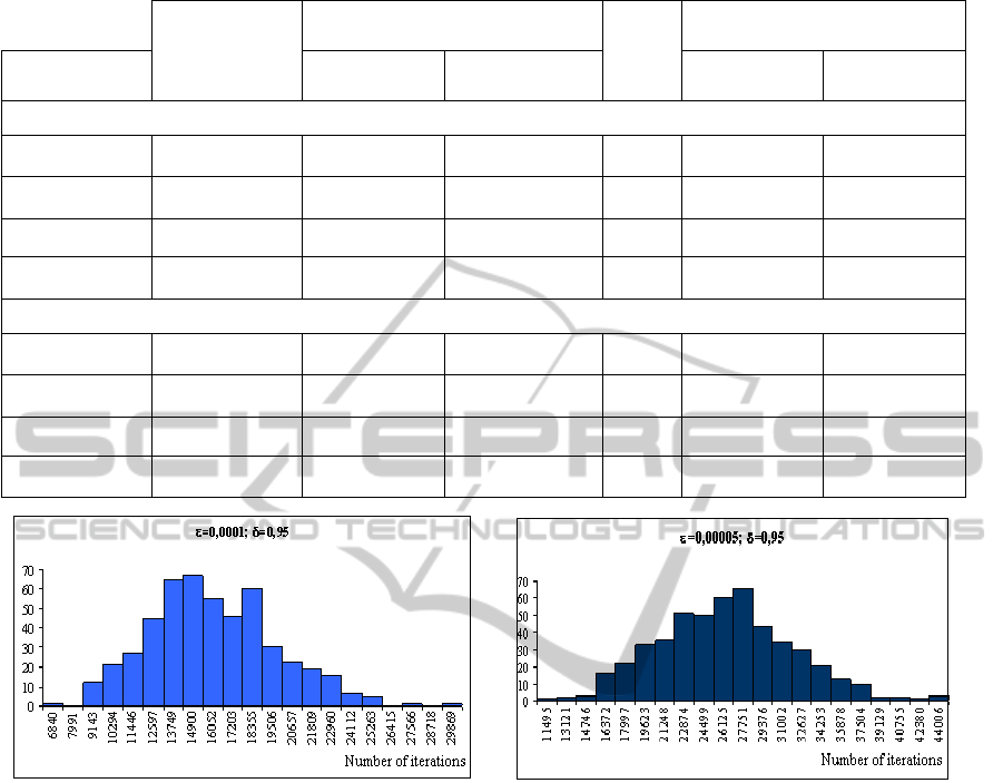
Table 1: Computer modelling results of the minimum value and the confidence interval.
kN
A
,
Confidence interval
p
Confidence interval of the hitting
probability p
Confidence
probability
Lower bound Upper bound Lower bound Upper bound
Example 1
9.0=
δ
-0.0000000307 -0.000000483 0.0000002275 0.91 0.8614377 0.94498488
95.0=
δ
0.0000000005 -0.00000002 0.0000000072 0.95 0.89763031 0.98009752
975.0=
δ
-0.000000031 -0.00000151 0.0000002275 0.98 0.92955759 0.9975685
99.0=
δ
-0.000000031 -0.00000239 0.0000002275 0.98 0.91852038 0.99850762
Example 2
9.0=
δ
0.0000478328 -0.00077633 0.000620020 0.886 0.90384692 0.86549069
95.0=
δ
0.0000478328 -0.00122913 0.000620020 0.948 0.92806921 0.96283961
975.0=
δ
0.0000478328 -0.00169791 0.000620020 0.97 0.95099096 0.98311659
99.0=
δ
0.0000478328 -0.00234306 0.000620020 0.984 0.96551508 0.99416328
Figure 7: The number of iterations after termination of the algorithm (two dimensional Iris Plant data).
6 CONCLUSIONS
A linear estimator and confidence bounds for the
minimum value of the function have been proposed,
using order statistics of the function values provided
by SA algorithm, which were studied in an
experimental way. These estimators are simple and
depend only on the parameter of the extreme value
distribution
α. The latter parameter α is easily
estimated, using the parameter of homogeneity of
the objective function or in a statistical way.
Theoretical considerations and computer examples
have shown that the confidence interval of the
function minimum can be estimated with an
admissible accuracy, when the number of iterations
is increased. Empirical study of the statistical
hypothesis on order statistics have shown that
function values lead us to a conclusion that the
estimates proposed can be applied in optimality
testing and termination of the SA algorithm. The
estimates introduced here can be used to create the
termination criterion for SA algorithm, namely, the
algorithm stops, when the length of the confidence
interval becomes smaller than prescribed value
0>
ε
.
REFERENCES
Astorino, A., Fuduli, A., 2007. Nonsmooth Optimization
Techniques for Semisupervised Classification.
IEEE
Transactions on Pattern Analysis and Machine
Intelligence, vol. 29, No. 12, p. 2135-2142.
Asuncion, A., Newman, D. J., 2007.
UCI Machine
Learning Repository
. School of Information and
Computer Science
, University of California, Irvine,
CA. (http://www.ics.uci.edu/˜mlearn/ MLRepository.
html)
TERMINATION OF SIMULATED ANNEALING ALGORITHM SOLVING SEMI-SUPERVISED LINEAR SVMS
PROBLEMS
155

Bartkutė, V., Sakalauskas, L., 2004. Order statistics for
testing optimality in stochastic optimization.
Proceedings of the 7
th
International Conference
Computer data analysis and Modelling”
, Minsk, p.
128-131
Bartkute, V., Sakalauskas, L., 2009a. Statistical Inferences
for Termination of Markov Type Random Search
Algorithms. Journal of Optimization Theory and
Applications
, vol. 141, p. 475-493.
Bartkutė-Norkuniene V., 2009b. Stochastic Optimization
Algorithms for Support Vector Machines
Classification.
Informatica, vol. 20, No. 2, p. 173–186.
Bennett, K. P., Demiriz, A., 1999. Semi-supervised
support vector machines. In M. S. Kearns, S. A. Solla,
and D. A. Cohn, editors,
NIPS, vol. 11, p. 368–374.
Cortes, C., Vapnik, V., 1995. Support-vector networks.
Machine Learning, vol. 20, No. 3, p. 273-297.
Galambosh, Y., 1984.
Asymptotic Theory of Extremal
Order Statistics
, Nauka, Moscow (in Russian).
Granville, V., Krivanek, M., Rasson, J. P., 1994.
Simulated annealing: a proof of convergence. IEEE
Transactions on Pattern Analysis and Machine
Intelligence, vol 16, No. 6, p. 652–656.
Hall, P., 1982. On estimating the endpoint of a
distribution. Annals of Statistic, vol. 10, p. 556-568.
Huang, T. M., Kecman, V., 2004. Semi-supervised
Learning from Unbalanced Labeled Data – An
Improvement, in 'Knowledge Based and Emergent
Technologies Relied Intelligent Information and
Engineering Systems', Eds. Negoita, M. Gh., at al.,
Lecture Notes on Computer Science, vol. 3215, p.
765-771.
Mockus, J., 1967. Multi-Extremal Problems in
Engineering Design
. Nauka, Moscow, (in Russian).
Yang, R. L., 2000. Convergence of the simulated
annealing algorithm for continuous global
optimization.
Journal of Optimization Theory and
Applications
, vol. 104, No. 3, p. 691–716.
Zilinskas, A., Zhigljavsky, A., 1991.
Methods of the
global extreme searching
. Nauka, Moscow, (in
Russian).
Zilinskas, A., Zhigljavsky, A., 2007.
Stochastic global
optimization
. Springer.
ICORES 2012 - 1st International Conference on Operations Research and Enterprise Systems
156
