
DETECTION AND RECOGNITION OF SUBPIXEL TARGETS
WITH HYPOTHESES DEPENDENT BACKGROUND POWER
Victor Golikov and Olga Lebedeva
Ingineering Faculty, Autonomous University of Carmen, 56 st., No. 4, Ciudad del Carmen, Camp., Mexico
Keywords: Statistical Detection and Recognition, Subpixel Targets.
Abstract: We consider the problem of detecting and recognizing the subpixel targets in sea background when the
background power may be different under the null hypothesis – where it is assumed to be known – and the
alternative multiple hypotheses. This situation occurs when the presence of the target triggers a decrease in
the background power (subpixel targets). We extend the formulation of the Matched Subspace Detector
(MSD) to the case where the background power is only known under the null hypothesis using the
generalized likelihood ratio test (GLRT) for the multiple hypotheses case. The obtained multiple hypotheses
test is based on the Modified MSD test (MMSD). We discuss the difference between the two detection and
recognition systems: based on the MSD and MMSD tests. Numerical simulations attest to the validity of the
performance analysis.
1 INTRODUCTION
Among the various frameworks in which pattern
recognition has been traditionally formulated, the
statistical approach has been most intensively
studied and used in practice (Webb, 2002). Target
detection and recognition in the remotely sensed
image sequences can be conducted spatially,
temporally or spectrally. The need for subpixel
temporally (or spectrally) detection-recognition in
remotely sensed image sequences arises from the
fact that the targets sampling distances are generally
larger than the sizes of targets of interest. In this
case, the target is embedded in a single pixel
sequence and cannot be detected or recognized
spatially. As a result, traditional spatial-temporal
analysis-based image sequence processing
techniques are not applicable. Matched subspace
detection-recognition is used to recognize the
mulptiple hypotheses of different targets presence or
absence of targets that are expected to lie in
particular subspaces of the measurements. Standard
approach in this case bases on calculating for each
possible target of the GLR and determination of the
target with maximum value of the GLR (Izenman,
2008). The common drawback of this approach is
the assumption that the background power under
hypothesis H
0
remains the same one as under
hypotheses H
k
. In digital optical systems, it is
typically that the background has the same
covariance structure under hypotheses H
0
and H
k
, but
different variances (Manolakis and Shaw, 2002),
which is directly related to the fill factor, that is, the
percentage of the pixel area occupied by the
background. Because the background power is
changed if any of the targets is present, the
detection-recognition system is not optimum and,
therefore, it is necessary to modify the MSD
(Golikov, Lebedeva 2011). As a result, we assume
that the proposed detection-recognition system can
achieve a significant performance advantage against
conventional one.
In this paper, we focus on the detection-
recognition of small targets in the case of unknown
power of Gaussian background under hypothesis H
i
.
We assume that different targets have the different
subspace dimensions. In section 2, we formulate the
subpixel detection-recognition problem using the
linear mixing model and the concepts of targets and
background subspaces. We derive the GLRT for the
problem at hand and the distributions under the
hypotheses. In Section 3, we investigated the
detection-recognition performance losses in the case
of background power variations between multiple
hypotheses in a Gaussian environment for proposed
and canonical detection-recognition systems in the
presence of a mismatch between the designed and
actual background power. Here, the numerical
simulations are included to verify the validity of the
555
Golikov V. and Lebedeva O. (2012).
DETECTION AND RECOGNITION OF SUBPIXEL TARGETS WITH HYPOTHESES DEPENDENT BACKGROUND POWER.
In Proceedings of the 1st International Conference on Pattern Recognition Applications and Methods, pages 555-558
DOI: 10.5220/0003756405550558
Copyright
c
SciTePress

theoretical analysis. Brief conclusions end the paper.
2 GENERALIZED LIKELIHOOD
RATIO TEST
The problem addressed here is the detection-
recognition of a K possible targets response s
k
for a
measurement x~N[
θ
k
,
R
2
k
σ
] in Gaussian
background with covariance structure
,R
2
k
σ
k=1,2,…,K. The problem is to decide between the
null hypothesis (H
0
) and the alternative hypotheses
(H
k
): H
0
: x=c
0
,
H
k
: x=µs
k
+c
k
. (1)
When the background covariance matrix R, scaling
, target subspace matrix H
k
, and the location
parameter θ
k
are known, the appropriate detection-
recognition statistics is presented in the MSD form
(Scharf, 1991):
T
kn
(x)
=(1/σ
)max
[
(
)
]
(
)
(2)
We accept the hypothesis H
k
when the statistics (2)
achieves the maximum. The parameter θ
k
locates the
target response μs
k
=
θ
k
in the target subspace
spanned by the p
k
<N columns of a known matrix
, H=
×
, which is the linear space of (N×p
k
)
complex matrices. Let define the whitened targets
mode matrix
=R
-1/2
and the whitened
measurements y=R
-1/2
x. We want to derive the
detection-recognition test in the case of unknown
parameters
using the generalized likelihood ratio
of the conditional probability density functions
(PDF). The maximized ratio of PDFs is obtained by
replacing the unknown parameters by their
estimators according to maximum likelihood (ML)
criterion in such form:
L=
,
;
,
;
⁄
=
max
,
[
exp(−(1/
)
(
−
)
(
−
)
)]
exp[−
1
]
,
(3)
where the numerator are maximized by parameter
σ
k
2
. The ML estimates (Jolliffe, 2002) of the
is
obtained by solving such equations:
=0.
(4)
We designate the target subspaces matrix with a
maximum number p
max
of columns as H
max
and
. It is well known (Scharf, 1991) that the
estimate of the background variance is obtained as:
=
,
(5)
where
= I-
and P
Φ
=
(
)
-1
.
Next, the maximum of (3) with respect to σ
k
2
is
found for
, resulting in
=max
()
(
)
.
(6)
Computing the logarithm of the N-th root of (6), we
obtain the decision statistics:
T
un
(y)=max
−
(
)
−1
=max
+
−
(
)
−1 ,
(7)
where A is the factor of the recognition sensitivity.
3 PERFORMANCE ANALYSIS
In this section, we derive the asymptotic distribution
of the test statistic T
un
with a view to evaluate it
performance in terms of probability of detection, the
probability of the recognition error and probability
of false alarm. Moreover, we analyze numerically
the difference of the performance between
conventional statistics T
kn
(x) and the proposed
statistics T
un
(x). It is well known that the distribution
of the statistics T
kn
(x) is following:
,
⎪
⎪
⎩
⎪
⎪
⎨
⎧
=
kkp
k
p
kn
H
N
H
N
T
k
k
under )(2
2
under
2
1
)(
2
2
0
2
0
2
2
λχ
σ
σ
χ
x
(8)
.
kk
H
k
H
k
k
k
θHRHθ
1
2
2
−
=
σ
μ
λ
(9)
By analogy, we observe that the first term in (7)
is equal to T
kn
(x), the second term has
(
)
central distribution with 2(N-p
k
) real degrees of
freedom under H
0
and
(
)
central
distribution under H
k
. In order to come up with
manageable expressions, we investigate an
asymptotic approach, assuming that the parameter N
is large. In this case, it is well known that the chi-
square distribution χ
n
2
(0) converges to a Gaussian
distribution with mean n and variance 2n (Scharf,
1991). Then, using the fact that the third term
Q(y)=
(
)
has the chi-square distribution,
ICPRAM 2012 - International Conference on Pattern Recognition Applications and Methods
556

one can write the following asymptotical expression:
Q()~
1,
under
,
under
,
(10)
where b
k
=
. Using a Taylor series expansion of
lnQ() around 1, it is easy to obtain that
Q(y)–1–ln[Q(y)] ≈ (1/2)[Q(y) -1]
2
. (11)
We used the latter approximation and found that
Q(y)–1-ln[Q(y)]
~
1
2(−
)
(
0
)
under
2(−
)
(−
)[
−1)]
under
.
(12)
Since the first term and Q(y) are independent, the
asymptotic distribution of T
un
(x) is given by as
follows:
(
)
~
1
2(−
)
(
0
)
+
1
2
(
0
)
2(−
)
(−
)(
−1)
+
2
(
2
)
.
The distributions derived above enable one to obtain
the receivers operating characteristics (ROC). In
order to come up with exploitable expressions, we
examine a further
approximation:
(
)
=
1
2
(
0
)
under
2
(
+
)
under
,
(13)
where
=
(
)
(
)
. This expression holds
for large N, p
k
<<N and b
k
=1-p
k
/N. One can calculate
the ROC using the following expression:
B(η, n, λ)=
(,)
()
.
(14)
Also, one can obtain the threshold
=
(,,) using its inverse function. Then,
the probability of false alarm F and probability of
detection D can be written in such form:
,0)12 ,(2)( +=
kun
pNηBTF
,
(15)
).,12 ,(2)(
0
1
kkkun
pbBTD
λλη
++=
−
(16)
If we fix the false alarm rate F it is obvious that the
increase of the factor of the detector sensitivity A
augments the threshold . In order to comprehend
how and why the proposed statistics T
un
may
outperform the T
kn
, let provide a qualitative analysis
of the differences between these systems. The T
kn
depends only on the data projection on the targets
subspaces; the proposed statistics T
un
depends on the
projection on the background subspace. Notice that
the only information used by T
un
to modify T
kn
is the
power in the background subspace. One can then
expect the different behavior of the T
un
, each time
the estimated background power is different from
the expected one. The projection onto the targets
subspaces will decrease and the projection onto the
background subspace will increase. The developed
system could recover a part of the energy having
moved from one subspace to the other and try to
maintain the test performance. Note that the
(
)
=
and then Δ
(
)
=
is approximately
zero for b=1, and is a monotonically increasing
function when the parameter b decreases. This
corrective termΔ
(
)
estimates the background
variance for H
k
and calculates the difference with the
presumed one (σ
0
2
). The mean of the statistics T
kn
diminishes under the assumption that the parameter
b decreases and then, when it is close to zero target
amplitude µ, the detection probability can be much
less than the presumed value of the false alarm
probability. Therefore, performance of the T
kn
suffers a remarkable degradation. The additional
corrective term Δ
(
)
increases the value of statistics
and, therefore, increases the probability of detection.
When the targets have the same size and hence the
same pixel fill factor b, the recognition performance
of the T
kn
and T
un
is approximately equal, but in the
case of the targets of the different size and therefore
with the different pixel fill factor the corrective term
Δ
(
)
is different and this term causes the decreases
the recognition errors. At the numerical analysis
stage, one should specify the background and target
models properties. Let model the target mode matrix
H is a Vandermonde matrix (Scharf, 1991). In the
literature, it is often assumed (Scharf, 1991) that
background has an exponential covariance matrix
structure with one-lag correlation coefficient ρ. The
parameter θ is unknown in practice but for our
scenario it is possible to use the appropriate
deterministic approximation
[]
T
1,,1,1 L=θ
. In order
to limit the computational burden, the false alarm
probability is chosen as F=10
-3
. Figs.1, 2 illustrate
the relation between the detection probability D and
signal-to-background ratio (
dB
2
0
2
σμ
) under the
chosen system constraint resulting from 10
6
Monte
Carlo trials. Comparing figures 1 and 2 we notice,
that the system in the case of the correlated
background with a known covariance matrix in
comparison with the uncorrelated one requires the
DETECTION AND RECOGNITION OF SUBPIXEL TARGETS WITH HYPOTHESES DEPENDENT BACKGROUND
POWER
557
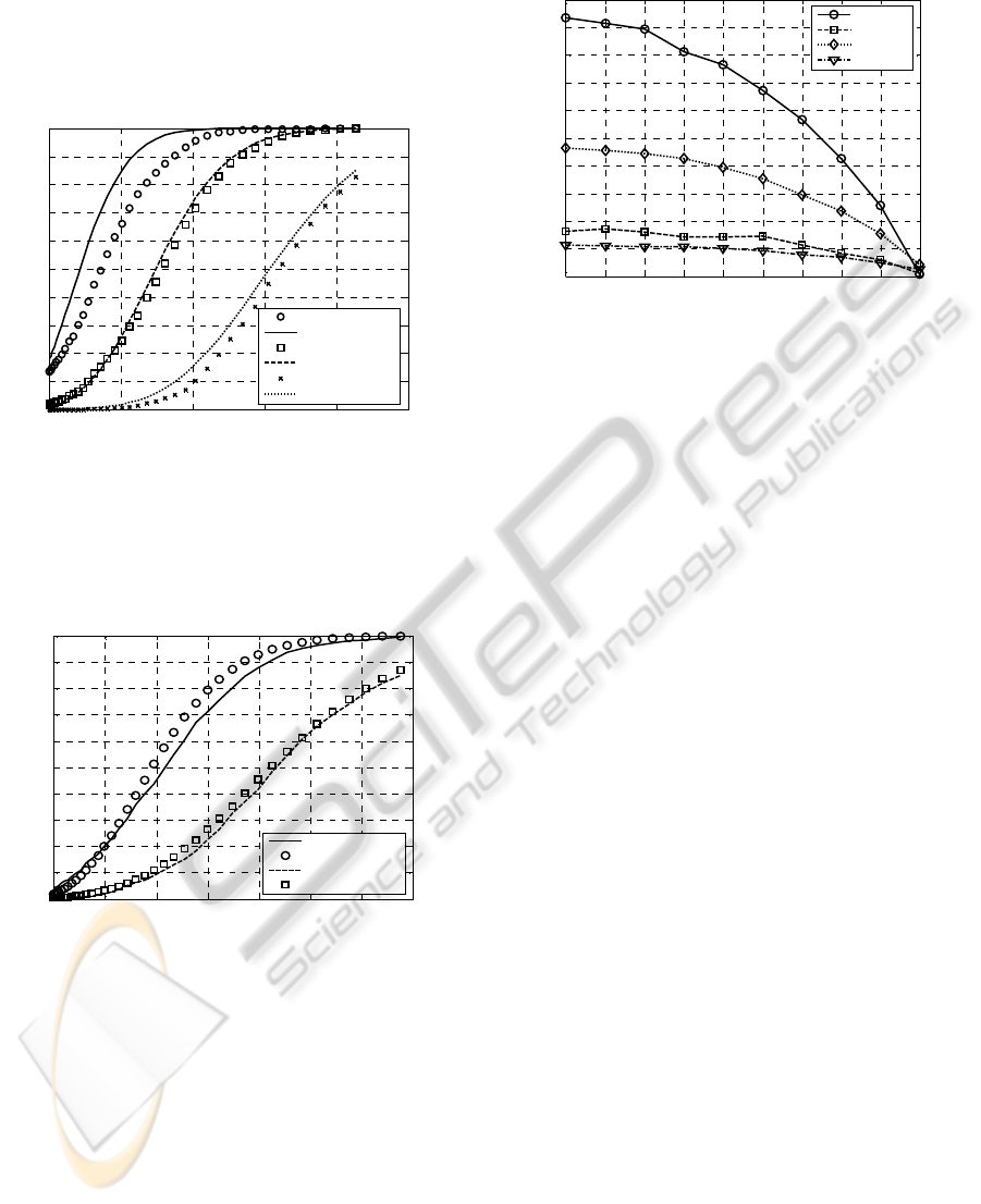
smaller SBR for achieving of good detection.
Recognition errors for different targets depend on
difference between their subspace dimensions. In
this example the recognition error between the first
target with p=5 and the second with p=20 is equal to
6% and between the first and third targets
Figure 1: Probability of detection versus SBR
in
for
proposed system for target fill factor
b =0.8. The lines
depict the analytical results, whereas the markers show
Monte Carlo simulation trial results. The false alarm rate
F=10
-3
, number of measurements N=200, 3 targets with
subspace dimensions:
p=5, 20, 50, uncorrelated
background
ρ= 0; A=1.
Figure 2: Probability of detection versus SBR
in
for
proposed system for target fill factor
b =0.8. The lines
depict the analytical results, whereas the markers show
Monte Carlo simulation trial results. The false alarm rate
F=10
-3
, number of measurements N=200, 2 targets with
subspace dimensions:
p=5 and 20, correlated background
ρ= 0.9; A=1.
about 2% in presence of uncorrelated background;
these errors is equal to 8% and 3% in presence of
correlated background with ρ= 0.9. The
figure 3
shows the comparison in the detectability by the two
systems. One can see that at the pixel fill factor b<1
the known system has losses in SBR with respect to
the proposed system. Quality of recognition by the
proposed system slightly is better, than by the
known system.
Figure 3: Loss factor of detection versus fill factor of
target
b for proposed system (ND) and well known
(MSD). 2 targets with dimensions:
p =10 and 40.
Simulation results for
F=10
-3
, number of measurements
N=200, uncorrelated background; A=1.
4 CONCLUSIONS
In this work, we intend to extend the detection-
recognition problem in the case of the subpixel
targets and Gaussian environment. We derived the
GLRT for the problem at hand and carried out a
performance analysis of the proposed system. The
synthesized system modifies the well known by
adding the corrective term proportional to the square
of the background power variation. This term
compensates a priori background power uncertainty
in the case of the target’s presence. It has been
shown analytically and via statistical simulation that
the performance of the proposed system
considerably outperforms the known system
performance.
REFERENCES
Webb, A., 2002. Statistical Pattern Recognition, Wiley.
NY. 2
nd
edition.
Izenman, A., 2008.
Modern Multivariate Statistical
Techniques: Regression, Classification, and Manifold
Manifold Learning,
Springer. NY.
Manolakis, D., and Shaw, G., 2002. Detection Algorithms
for Hyperspectral Imaging Applications. IEEE Signal
Processing Magazine.
Vol. 19, no. 1, pp. 29-43.
Golikov, V., Lebedeva, O., Castillejos-Moreno, A., and
Ponomaryov, V., 2011. Performance of the Matched
Subspace Detector in the case of Subpixel Targets.
IEICE Trans. Fund. Vol. E94-A, no. 2, pp. 826-828.
Scharf, L., 1991.
Statistical Signal Processing, Addison-
Wesley, NY.
0 0.05 0.1 0.15 0.2 0.25
0
0.1
0.2
0.3
0.4
0.5
0.6
0.7
0.8
0.9
1
Probability of detection
Signal-to-background ratio
Sim., p=5, b=0.8
Theor.,p=5, b=0.8
Sim., p=20, b=0.8
Theor., p=20, b=0.8
Sim., p=50, b=0.8
Theor., p=50, b=0.8
0 1 2 3 4 5 6 7
x 10
-3
0
0.1
0.2
0.3
0.4
0.5
0.6
0.7
0.8
0.9
1
Signal-to-background ratio
Probability of detection
Theor., b=0.8, p=5
Sim., b=0.8, p=5
Theor., b=0.8, p=20
Sim., b=0.8, p=20
0.1 0.2 0.3 0.4 0.5 0.6 0.7 0.8 0.9 1
0
0.5
1
1.5
2
2.5
3
3.5
4
4.5
5
Fill factor b
Loss factor (dB)
MSD, p=40
ND, p=40
MSD, p=10
ND, p=10
ICPRAM 2012 - International Conference on Pattern Recognition Applications and Methods
558
