CLASSIFICATION OF 3D URBAN SCENES

A Voxel based Approach

Ahmad Kamal Aijazi

1,2

, Paul Checchin

1,2

and Laurent Trassoudaine

1,2

Clermont Universit´e, Universit´e Blaise Pascal, Institut Pascal, BP 10448, F-63000 Clermont-Ferrand, France

CNRS, UMR 6602, Institut Pascal, F-63171 Aubiere, France

Keywords:

3D point cloud segmentation, Hybrid data, Super-Voxels, Urban scene classiﬁcation.

Abstract:

In this paper we present a method to classify urban scenes based on a super-voxel segmentation of sparse 3D

data. The 3D point cloud is ﬁrst segmented into voxels, which are then joined together by using a link-chain

method rather than the usual region growing algorithm to create objects. These objects are then classiﬁed

using geometrical models and local descriptors. In order to evaluate our results a new metric is presented,

which combines both segmentation and classiﬁcation results simultaneously. The effects of voxel size and

incorporation of RGB color and intensity on the classiﬁcation results are also discussed.

1 INTRODUCTION

The automatic segmentation and classiﬁcation of 3D

urban data have gained widespread interest and im-

portance in the scientiﬁc community due to the in-

creasing demand of urban landscape analysis and car-

tography for different popular applications, coupled

with the advances in 3D data acquisition technology.

The automatic extraction (or partially supervised) of

important urban scene structures such as roads, veg-

etation, lamp posts, and buildings from 3D data has

been found to be an attractive approach to urban scene

analysis because it can tremendously reduce the re-

sources required in analyzing the data for subsequent

use in 3D city modeling and other algorithms.

A common way to quickly collect 3D data of

urban environments is by using an airborne LiDAR

(Sithole and Vosselman, 2004), (Verma et al., 2006),

where the LiDAR scanner is mounted in the bottom of

an aircraft. Although this method generates a 3D scan

in a very short time period, there are a number of lim-

itations in 3D urban data collected from this method

such as a limited viewing angle.

These limitations are overcome by using a mobile

terrestrial or ground based LiDAR system in which

unlike the airborne LiDAR system, the 3D data ob-

tained is dense and the point of view of the images

is closer to the urban landscapes. However this of-

fers both advantages and disadvantages when pro-

cessing the data. The disadvantages include the de-

mand for more processing power required to handle

the increased volume of 3D data. On the other hand,

the advantage is the availability of a more detailed

sampling of the object’s lateral views, which provides

a more comprehensive model of the urban structures

including building facades, lamp posts, etc.

Our work revolves around the segmentation and

then classiﬁcation of ground based 3D data of ur-

ban scenes. The aim is to provide an effective pre-

processing step for different subsequent algorithms or

as an add-on boost for more speciﬁc classiﬁcation al-

gorithms.

2 RELATED WORK

In order to fully exploit3D point clouds, effective seg-

mentation has proved to be a necessary and critical

pre-processing step in a number of autonomous per-

ception tasks.

Earlier works including (Anguelov et al., 2005),

(Lim and Suter, 2007) and (Munoz et al., 2009) used

small sets of specialized features, such as local point

density or height from the ground, to discriminate

only few object categories in outdoor scenes, or to

separate foreground from background. Lately, seg-

mentation has been commonly formulated as graph

clustering. Instances of such approaches are Graph-

Cuts including Normalized-Cuts and Min-Cuts.

(Golovinskiy and Funkhouser, 2009) extended

Graph-Cuts segmentation to 3D point clouds by us-

Aijazi A., Checchin P. and Trassoudaine L. (2012).

CLASSIFICATION OF 3D URBAN SCENES - A Voxel based Approach.

In Proceedings of the 1st International Conference on Pattern Recognition Applications and Methods, pages 61-70

DOI: 10.5220/0003733100610070

 SciTePress

ing k-Nearest Neighbors (k-NN) to build a 3D graph.

In this work edge weights based on exponential decay

in length were used. But the limitation of this method

is that it requires prior knowledge of the location of

the objects to be segmented.

Another segmentation algorithm for natural im-

ages, recently introduced by Felzenszwalb and Hut-

tenlocher (FH) (Felzenszwalb and Huttenlocher,

2004), has gained popularity for several robotic ap-

plications due to its efﬁciency. (Zhu et al., 2010) pre-

sented a method in which a 3D graph is built with

k-NN while assuming the ground to be ﬂat for re-

moval during pre-processing. 3D partitioning is then

obtained with the FH algorithm. We have used the

same assumption.

(Triebel et al., 2010) modiﬁed the FH algorithm

for range images to propose an unsupervised proba-

bilistic segmentation technique. In this approach, the

3D data is ﬁrst over-segmentedduringpre-processing.

(Schoenberg et al., 2010) have applied the FH al-

gorithm to colored 3D data obtained from a co-

registered camera laser pair. The edge weights are

computed as a weighted combination of Euclidean

distances, pixel intensity differences and angles be-

tween surface normals estimated at each 3D point.

The FH algorithm is then run on the image graph to

provide the ﬁnal 3D partitioning. The evaluation of

the algorithm is done on road segments only.

(Strom et al., 2010) proposed a similar approach

but modiﬁed the FH algorithm to incorporate angle

differences between surface normals in addition to the

differences in color values. Segmentation evaluation

was done visually without ground truth data. Our

approach differs from the above mentioned methods

as, instead of using the properties of each point for

segmentation resulting in over segmentation, we have

grouped the 3D points based on Euclidian distance

into voxels and then assigned normalized properties

to these voxels transforming them into super-voxels.

This not only prevents over segmentation but in fact

reduces the data set by many folds thus reducing post-

processing time.

A spanning tree approach to the segmentation

of 3D point clouds was proposed in (Pauling et al.,

2009). Graph nodes represent Gaussian ellipsoids as

geometric primitives.

These ellipsoids are then merged using a tree

growing algorithm. The resulting segmentation is

similar to a super-voxel type of partitioning with vox-

els of ellipsoidal shapes and various sizes. Unlike

this method, our approach uses cuboids of different

shapes and sizes as geometric primitives and a link-

chain method to group them together. In the litera-

ture survey we also ﬁnd some segmentation methods

based on surface discontinuities such as (Moosmann

et al., 2009) who used surface convexity in a terrain

mesh as a separator between objects.

In the past, research related to 3D urban scene

classiﬁcation and analysis had been mostly performed

using either 3D data collected by airborne LiDAR

for extracting bare-earth and building structures (Lu

et al., 2009) (Vosselman et al., 2005) or 3D data col-

lected from static terrestrial laser scanners for extrac-

tion of building features such as walls and windows

(Pu and Vosselman, 2009). In (Lam et al., 2010) the

authors extracted roads and objects just around the

roads like road signs. They used a least square ﬁt

plane and RANSAC method to ﬁrst extract a plane

from the points followed by a Kalman ﬁlter to ex-

tract roads in an urban environment. A method of

classiﬁcation based on global features is presented in

(Halma et al., 2010) in which a single global spin

image for every object is used to detect cars in the

scene while in (Rusu et al., 2010) a Fast Point Fea-

ture Histogram (FPFH) local feature is modiﬁed into

global feature for simultaneous object identiﬁcation

and view-point detection. Classiﬁcation using local

features and descriptors such as Spin Image (John-

son, 1997), Spherical Harmonic Descriptors (Kazh-

dan et al., 2003), Heat Kernel Signatures (Sun et al.,

2009), Shape Distributions (Osada et al., 2002), 3D

SURF feature (Knopp et al., 2010) is also found in

the literature survey. There is also a third type of

Classiﬁcation based on Bag Of Features (BOF) as dis-

cussed in (Liu et al., 2006). In (Lim and Suter, 2008)

a method of multi-scale Conditional Random Fields

is proposed to classify 3D outdoor terrestrial laser

scanned data by introducing regional edge potentials

in addition to the local edge and node potentials in

the multi-scale Conditional Random Fields. This is

followed by ﬁtting plane patches onto the labeled ob-

jects such as building terrain and ﬂoor data using the

RANSAC algorithm as a post-processing step to ge-

ometrically model the scene. (Douillard et al., 2009)

presented a method in which 3D points are projected

on to the image to ﬁnd regions of interest for classiﬁ-

cation.

In our work we use geometrical models based on

local features and descriptors to successfully classify

different segmented objects represented by groups of

voxels in the urban scene. Ground is assumed to be

ﬂat and is used as an object separator. Our segmen-

tation technique is discussed in Section 3. Section 4

deals with the classiﬁcation of these segmented ob-

jects. In Section 5 a new evaluation metric is intro-

duced to evaluate both segmentation and classiﬁca-

tion together while in Section 6 we present the results

of our work. Finally, we conclude in Section 7.

ICPRAM 2012 - International Conference on Pattern Recognition Applications and Methods

3 VOXEL SEGMENTATION

3.1 Voxelisation of Data

When dealing with large 3D data sets, the computa-

tional cost of processing all the individual points is

very high, making it unpractical for real time applica-

tions. It is therefore sought to reduce these points by

grouping or removing redundant or un-useful points

together. Similarly, in our work the individual 3D

points are clustered together to form a higher level

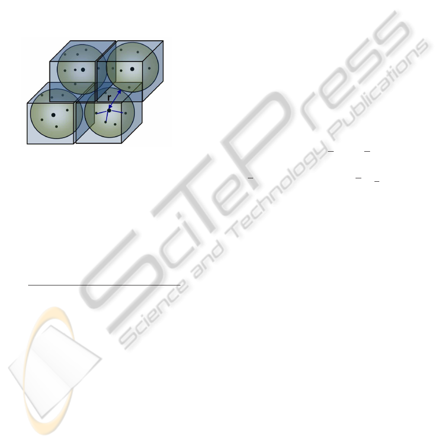
representation or voxel as shown in Figure 1.

Figure 1: A number of points is grouped together to form

cubical voxels of maximum size 2r. The actual voxel sizes

vary according to the maximum and minimum values of the

neighboring points found along each axis to ensure the pro-

ﬁle of the structure.

For p data points, a number of s voxels, where

s << p, are computed based on k-NN with w = 1/d

given as the weight to each neighbor (where d is the

distance to the neighbor). Let P and Q be two points

in the X, Y and Z coordinate system then d is given

as:

d =

−Q

)

+ (P

−Q

)

+ (P

−Q

)

(1)

The maximum size of the voxel 2r, where r is ra-

dius of ellipsoid, depends upon the density of the 3D

point cloud. In (Lim and Suter, 2008) color values are

also added in this step but it is observed that for rel-

atively smaller voxel sizes, the variation in properties

such as color is not much and just increases computa-

tional cost. For these reasons we have only used dis-

tance as a parameter in this step and the other proper-

ties in the next step of clustering the voxels to form

objects. Also we have ensured that each 3D point

which belongs to a voxel is not considered for further

voxelisation. This not only prevents over segmenta-

tion but also reduces processing time.

For the voxels we use a cuboid because of its sym-

metry which avoids ﬁtting problems while grouping

and also minimizes the effect of voxel shape during

feature extraction.

Although the maximum voxel size is predeﬁned,

the actual voxel sizes vary according to the maximum

and minimum values of the neighboring points found

along each axis to ensure the proﬁle of the structure.

Once these voxels are created we ﬁnd the proper-

ties of each voxel. These properties include surface

normals, RGB-color, intensity, geometric primitives

such as barycenter, geometrical center, maximum and

minimum values along each axis, etc. Where some of

these properties are averaged and normalized values

of the constituting points, the surface normals are cal-

culated using PCA (Principal Component Analysis).

The PCA method has been proved to perform better

than the area averaging method (Klasing et al., 2009)

to estimate the surface normal.

Given a point cloud data set D = {x

}

i=1

, the PCA

surface normal approximation for a given data point

p ∈ D is typically computed by ﬁrst determining the

k-Nearest Neighbors, x

∈ D , of p. Given the K

neighbors, the approximate surface normal is then the

eigenvector associated with the smallest eigenvalue of

the symmetric positive semi-deﬁnite matrix

P =

∑

k=1

− p)

− p) (2)

where p is the local data centroid: p =

∑

j=1

The estimated surface normal is ambiguous in

terms of sign; to account for this ambiguity the dot

product between estimated surface normals is re-

peated using the negative estimated surface normal

of one of the vectors and the minimum result of the

term is selected. Yet for us the sign of the normal

vector is not important as we are more interested in

the orientation. Using this method, a single surface

normal is estimated for all the points belonging to a

voxel and is then associated with that particular voxel

along with the other properties, transforming it into a

super-voxel.

All these properties would then be used in group-

ing these super-voxelsinto objects and then during the

classiﬁcation of these objects. Instead of using thou-

sands of points in the data set, the advantage of this

approach is that we can now use the reduced number

of super-voxels to obtain similar results for classiﬁca-

tion and other algorithms. In our case, the data sets

of 110, 392, 53,676 and 27,396 points were reduced

to 18,541, 6,928 and 7,924 super-voxels respectively

which were then used for subsequent processing.

3.2 Clustering by Link-chain Method

When the 3D data is converted into super-voxels, the

next step is to group these super-voxels to segment

into distinct objects.

CLASSIFICATION OF 3D URBAN SCENES - A Voxel based Approach

Usually for such tasks a region growing algorithm

(Vieira and Shimada, 2005) is used in which the prop-

erties of the whole growing region may inﬂuence

the boundary or edge conditions. This may some-

times lead to erroneous segmentation. Also com-

mon in such type of methods is a node based ap-

proach (Moosmann et al., 2009) in which at every

node, boundary conditions have to be checked in all

5 different possible directions. In our work we have

proposed a link-chain method instead to group these

super-voxels together into segmented objects.

In this method each super-voxel is considered as a

link of a chain. All secondary links attached to each

of these principal links are found. In the ﬁnal step

all the principal links are linked together to form a

continuous chain removing redundantsecondary links

in the process as shown in Figure 2.

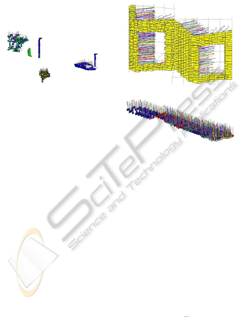
(a) (b) (c)

(d)

Figure 2: Clustering of super-voxels using a link-chain

method is demonstrated. (a) shows super-voxel 1 taken as

principal link in red and all secondary links attached to it

in blue. (b) and (c) shows the same for super-voxel 2 and

3 taken as principal links. (d) shows the linking of princi-

pal links (super-voxels 1, 2 & 3) to form a chain removing

redundant secondary links.

Let V

be a principal link and V

be the n number

of secondary links then each of the V

is linked to

if and only if the following three conditions are

fulﬁlled:



X,Y,Z

−V

X,Y,Z



≤ (w

+ c

) (3)



R,G,B

−V

R,G,B



≤ 3

√

(4)

−V

| ≤ 3

√

(5)

where, for the principal and secondary link super-

voxels respectively:

• V

X,Y,Z

, V

X,Y,Z

are the geometrical centers;

• V

R,G,B

, V

R,G,B

are the mean RGB values;

• V

, V

are the mean intensity values;

• w

is the color weight equal to the maximum

value of the variances Var(R,G,B);

• w

is the intensity weight equal to the maximum

value of the variances Var(I).

is the distance weight given as



X,Y,Z



. Here s

X,Y,Z

is the voxel size

along X, Y & Z axis respectively.

is the inter-distance constant (along the three

dimensions) added depending upon the density of

points and also to overcome measurement errors,

holes and occlusions, etc. The value of c

needs to

be carefully selected depending upon the data.

The orientation of normals is not considered in

this stage to allow the segmentation of complete ob-

jects as one entity instead of just planar faces.

This segmentation method ensures that only the

adjacent boundary conditions are considered for seg-

mentation with no inﬂuence of a distant neighbor’s

properties. This may prove to be more adapted to

sharp structural changes in the urban environment.

The segmentation algorithm is summarized in Algo-

rithm 1.

Algorithm 1: Segmentation.

1: repeat

2: Select a 3D point for voxelisation

3: Find all neighboring points to be included in

the voxel using k-NN within the maximum

voxel length speciﬁed

4: Find all properties of the super-voxel including

surface normal found by using PCA

5: until all 3D points are used in a voxel

6: repeat

7: Specify a super-voxel as a principal link

8: Find all secondary links attached to the princi-

pal link

9: until all super-voxels are used

10: Link all principal links to form a chain removing

redundant links in the process

With this method 18,541, 6,928 and 7,924 super-

voxels obtained from processing 3 different data sets

were successfully segmented into 237, 75 and 41 dis-

tinct objects respectively.

4 CLASSIFICATION OF

OBJECTS

In order to classify these objects, we assume the

ground to be ﬂat and use it as separator between ob-

jects. For this purpose we ﬁrst classify and segment

out the ground from the scene and then the rest of

ICPRAM 2012 - International Conference on Pattern Recognition Applications and Methods

the objects. This step leaves the remaining objects as

if suspended in space, i.e distinct and well separated,

making them easier to be classiﬁed as shown in Fi-

gure 3.

Figure 3: Segmented objects in a scene with prior ground

removal.

The ground or roads followed by these objects are

then classiﬁed using geometrical and local descrip-

tors. These mainly include:

a. Surface Normals. The orientation of the surface

normals is essential for classiﬁcation of ground

and building faces. For ground object the surface

normals are along Z-axis (height axis) whereas for

building faces the surface normals are parallel to

the X-Y axis (ground plane), see Figure 4.

b. Geometrical Center and Barycenter. The height

difference between the geometrical center and the

barycenter along with other properties is very use-

ful in distinguishing objects like trees and vegeta-

tion, etc., where:

h(barycenter−geometrical center) > 0

with h being the height function.

c. Color and Intensity. Intensity and color are also

an important discriminating factor for several ob-

jects.

d. Geometrical Shape. Along with the above men-

tioned descriptors, geometrical shape plays an im-

portant role in classifying objects. In 3D space,

where pedestrians and pole are represented as

long and thin with poles being longer, cars and

vegetation are broad and short. Similarly, as roads

represent a low ﬂat plane, the buildings are repre-

sented as large (both in width and height) vertical

blocks.

Using these descriptors we successfully classify

urban scenes into 5 different classes (mostly present

in our scenes) i.e. buildings, roads, cars, poles and

trees. The classiﬁcation results and a new evaluation

metric are discussed in the following sections.

(a) Normals of building.

(b) Normals of road.

Figure 4: (a) shows surface normals of building super-

voxels are parallel to the ground plane. In (b) it can be

clearly seen that the surface normals of road surface super-

voxels are perpendicular to the ground plane.

5 EVALUATION METRICS

In previous works, different evaluation metrics are in-

troduced for both segmentation results and classiﬁers

independently. Thus in our work we present a new

evaluation metric which incorporates both segmenta-

tion and classiﬁcation together.

The evaluation method is based on comparing the

total percentage of super-voxels successfully classi-

ﬁed as a particular object. Let T

, i ∈ {1,··· ,N},

be the total number of super-voxels distributed into

objects belonging to N number of different classes,

i.e this serves as the ground truth, and let t

, i ∈

{1,··· ,N}, be the total number of super-voxelsclassi-

ﬁed as a particular class of type-j and distributed into

objects belonging to N different classes (for example

a super-voxel classiﬁed as part of the building class

may actually belong to a tree) then the ratio S

(j is

the class type as well as the row number of the matrix

and k ∈{1, ··· , N}) is given as:

These values of S

are calculated for each type of

CLASSIFICATION OF 3D URBAN SCENES - A Voxel based Approach

class and are used to ﬁll up each element of the confu-

sion matrix, row by row (refer to Table 1 for instance).

Each row of the matrix represents a particular class.

Thus, for a class of type-1 (i.e. ﬁrst row of the

matrix) the values of:

True Positive rate, TP = S

(i.e the diagonal of the

matrix represents the TPs)

False Positive rate, FP =

∑

m=2

True Negative rate, TN = (1−FP)

False Negative rate, FN = (1−TP)

The diagonal of this matrix or TPs gives the Seg-

mentation ACCuracy SACC, similar to the voxel

scores recently introduced by (Douillard et al., 2011).

The effects of unclassiﬁed super-voxels are automati-

cally incorporated in the segmentation accuracy. Us-

ing the above values the Classiﬁcation ACCuracy

CACC is given as:

CACC =

TP+ TN

TP+ TN+ FP+ FN

(6)

This value of CACC is calculated for all N types

of classes of objects present in the scene. Overall

Classiﬁcation ACCuracy OCACC can then be calcu-

lated as

OCACC =

∑

i=1

CACC

(7)

where N is the total number of object classes present

in the scene. Similarly, the Overall Segmentation AC-

Curacy OSACC can also be calculated.

The values of T

and t

used above are laboriously

calculated by hand matching the voxeliseddata output

and the ﬁnal classiﬁed super-voxels and points.

6 RESULTS

Our algorithm was validated on 3D data acquired

from different urban scenes on the Campus of Univer-

sity Blaise Pascal in Clermont-Ferrand, France. The

results of three such data sets are discussed here. The

data sets consisted of 27,396, 53, 676 and 110,392

3D points respectively. These 3D points were cou-

pled with corresponding RGB and intensity values.

The results are now summarized.

6.1 Data Set 1

The data set consisting of 27,396 data points was re-

duced to 7,924 super-voxels keeping maximum voxel

size 0.3 m and c

= 0.25 m. These super-voxels are

then segmented into 41 distinct objects. The classiﬁ-

cation result of these objects is shown in Figure 5 and

in Table 1.

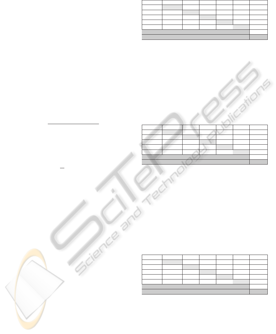
Table 1: Classiﬁcation results of data set 1 in the new eval-

uation metrics.

Building Road Tree Pole Car CACC

Building 0.943 0.073 0 0 0 0.935

Road 0.007 0.858 0.015 0.008 0 0.914

Tree 0 0.025 0.984 0 0 0.979

Pole 0 0.049 0 0.937 0 0.944

Car – – – – – –

Overall segmentation accuracy: OSACC 0.930

Overall classiﬁcation accuracy: OCACC 0.943

6.2 Data Set 2

The data set consisting of 53,676 data points was re-

duced to 6,928 super-voxels keeping maximum voxel

size 0.3 m and c

= 0.25 m. These super-voxels are

then segmented into 75 distinct objects. The classiﬁ-

cation result of these objects is shown in Figure 6 and

in Table 2.

Table 2: Classiﬁcation results of data set 2 in the new eval-

uation metrics.

Building Road Tree Pole Car CACC

Building 0.996 0.007 0 0 0 0.995

Road 0 0.906 0.028 0.023 0.012 0.921

Tree 0 0.045 0.922 0 0 0.938

Pole 0 0.012 0 0.964 0 0.976

Car 0 0.012 0 0 0.907 0.947

Overall segmentation accuracy: OSACC 0.939

Overall classiﬁcation accuracy: OCACC 0.955

6.3 Data Set 3

The data set consisting of 110,392 data points was

reduced to 18, 541 super-voxels keeping maximum

voxel size 0.3 m and c

= 0.25 m. These super-

voxels are then segmented into 237 distinct objects.

The classiﬁcation result of these objects is shown in

Figure 7 and in Table 3.

Table 3: Classiﬁcation results of data set 3 in the new eval-

uation metrics.

Building Road Tree Pole Car CACC

Building 0.901 0.005 0.148 0 0 0.874

Road 0.003 0.887 0.011 0.016 0.026 0.916

Tree 0.042 0.005 0.780 0 0 0.867

Pole 0 0.002 0 0.966 0 0.982

Car 0 0.016 0.12 0 0.862 0.863

Overall segmentation accuracy: : OSACC 0.879

Overall classiﬁcation accuracy: OCACC 0.901

6.4 Effect of Voxel Size on Classiﬁcation

Accuracy

As the properties of super-voxels are constant mainly

over the whole voxel length and these properties

are then used for segmentation and then classiﬁca-

tion, thus their size impacts the classiﬁcation process.

However as the voxel size changes, the inter-distance

constant c

also needs to be adjusted accordingly.

ICPRAM 2012 - International Conference on Pattern Recognition Applications and Methods

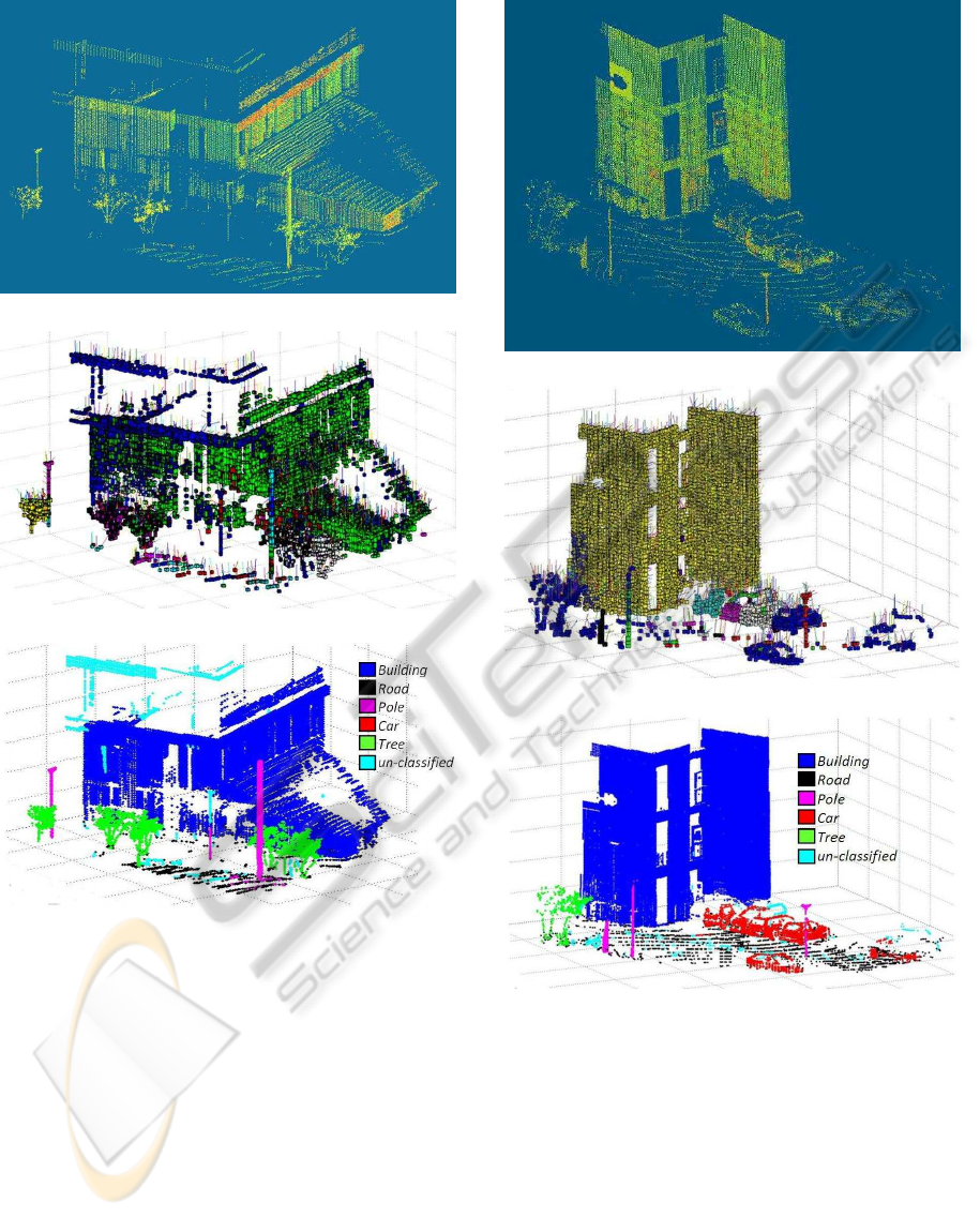
(a) 3D data points.

(b) Voxelisation and segmentation into objects.

Figure 5: (a) Shows 3D data points of data set 1. (b) shows

segmentation of 3D points. (c) shows classiﬁcation results

(labeled 3D points).

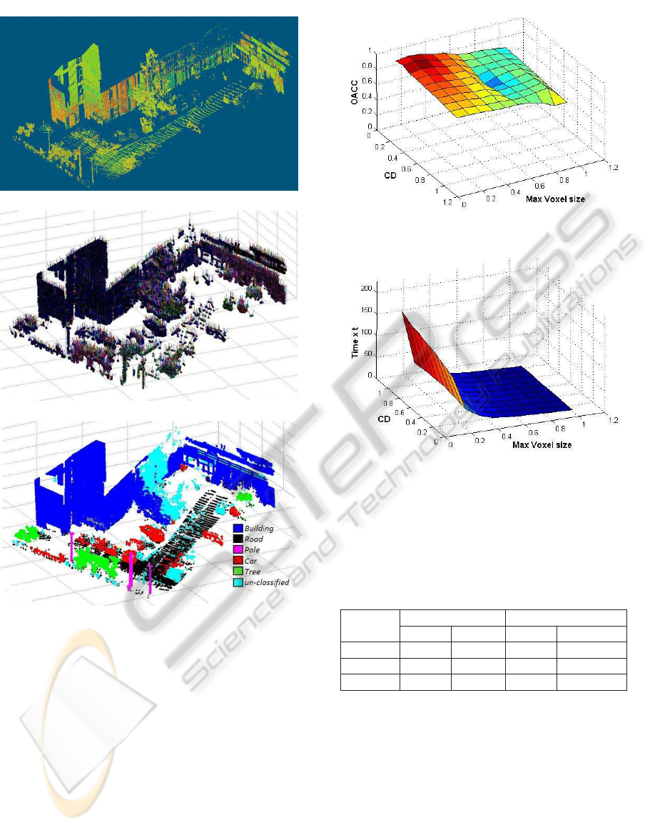
The effect of voxel size on the classiﬁcation result

was studied. The maximum voxel size and the value

of c

was varied from 0.1 m to 1.0 m on data set-1

and corresponding classiﬁcation accuracy was calcu-

lated. The results are shown in Figure 8(a). Then for

the same variation of maximum voxel size and c

the

variation in processing time was studied as shown in

Figure 8(b).

An arbitrary value of time T

is chosen for com-

parison purposes (along Z-axis time varies from 0 to

200T

). This makes the comparison results indepen-

dent of the processor used, even though the same pro-

(a) 3D data points.

(b) Voxelisation and segmentation into objects.

Figure 6: (a) Shows 3D data points of data set 2. (b) shows

segmentation of 3D points. (c) shows classiﬁcation results

(labeled 3D points).

cessor was used for all computations.

The results show that with smaller voxel size the

segmentation and classiﬁcation results improve (with

a suitable value of c

) but the computational cost in-

creases. It is also evident that variation in value of c

has no signiﬁcant impact on time t. It is also observed

that after a certain reduction in voxel size the classi-

ﬁcation result does not improve much but the com-

putational cost continues to increase manifolds. As

CLASSIFICATION OF 3D URBAN SCENES - A Voxel based Approach

(a) 3D data points.

(b) Voxelisation and segmentation into objects.

Figure 7: (a) Shows 3D data points of data set 3. (b) shows

segmentation of 3D points. (c) shows classiﬁcation results

(labeled 3D points).

both OCACC and time (both plotted along Z-axis)

are independent thus using and combining the results

of the two 3D plots in Figure 8 we can ﬁnd the opti-

mal value (in terms of OCACC and t) of maximum

voxel size and c

depending upon the ﬁnal applica-

tion requirements. For our work we have chosen a

maximum voxel size of 0.3 m and c

= 0.25 m.

6.5 RGB Color and Intensity

The effect of incorporating RGB Color and Intensity

on the segmentation and classiﬁcation results was also

studied. The results are presented in Table 4.

(a) Inﬂuence of voxel size on OCACC.

(b) Inﬂuence of voxel size on processing time.

Figure 8: (a) is a 3D plot in which the effect of maximum

voxel size and variation on OCACC is shown. In (b) the

effect of maximum voxel size and variation on processing

time is shown. Using the two plots we can easily ﬁnd the

optimal value for maximum voxel size and c

Table 4: Overall segmentation and classiﬁcation accuracies

when using RGB-Color and intensity values.

Data Set

Only RGB-Color Intensity with RGB-Color

OSACC OCACC OSACC OCACC

1 0.660 0.772 0.930 0.943

2 0.701 0.830 0.939 0.955

3 0.658 0.766 0.879 0.901

It is observed that incorporating RGB color alone

is not sufﬁcient in an urban environment due to the

fact that it is heavily affected by illumination variation

(part of an object may be under shade or reﬂect bright

sunlight) even in the same scene. This deteriorates

the segmentation process and hence the classiﬁcation.

This is perhaps responsible for the lower classiﬁcation

accuracy as seen in ﬁrst part of Table 4. It is the rea-

son why intensity values are incorporated as they are

illumination invariant and found to be more consis-

tent. The improved classiﬁcation results are presented

in second part of Table 4.

ICPRAM 2012 - International Conference on Pattern Recognition Applications and Methods

7 CONCLUSIONS

In this work we have presented a super-voxel based

segmentation and classiﬁcation method for 3D urban

scenes. For segmentation a link-chain method is pro-

posed, which is followed by a classiﬁcation of objects

using local descriptors and geometrical models. In

order to evaluate our work we have introduced a new

evaluation metric which incorporates both segmenta-

tion and classiﬁcation results. The results show an

overall segmentation accuracy of 87% and a classiﬁ-

cation accuracy of about 90%.

Our study shows that the classiﬁcation accuracy

improves by reducing voxel size (with an appropriate

value of c

) but at the cost of processing time. Thus

a choice of an optimal value, as discussed, is recom-

mended.

The study also demonstrates the importance of us-

ing intensity values along with RGB colors in the seg-

mentation and classiﬁcation of urban environment as

they are illumination invariant and more consistent.

The proposed method can also be used as an add-

on boost for other classiﬁcation algorithms.

ACKNOWLEDGEMENTS

This work is supported by the Agence Nationale de

la Recherche (ANR - the French national research

agency) (ANR CONTINT iSpace&Time – ANR-10-

CONT-23) and by “le Conseil G´en´eral de l’Allier”.

The authors would like to thank Pierre Bonnet and all

the other members of Institut Pascal who contributed

to this project.

REFERENCES

Anguelov, D., Taskar, B., Chatalbashev, V., Koller, D.,

Gupta, D., Heitz, G., and Ng, A. (2005). Discrim-

inative Learning of Markov Random Fields for Seg-

mentation of 3D Scan Data. In Computer Vision and

Pattern Recognition, IEEE Computer Society Confer-

ence on, volume 2, pages 169–176, Los Alamitos, CA,

USA. IEEE Computer Society.

Douillard, B., Brooks, A., and Ramos, F. (2009). A 3D

Laser and Vision Based Classiﬁer. In 5th Int. Conf. on

Intelligent Sensors, Sensor Networks and Information

Processing (ISSNIP), page 6, Melbourne, Australia.

Douillard, B., Underwood, J., Kuntz, N., Vlaskine, V.,

Quadros, A., Morton, P., and Frenkel, A. (2011). On

the Segmentation of 3D LIDAR Point Clouds. In

IEEE Int. Conf. on Robotics and Automation (ICRA),

page 8, Shanghai, China.

Felzenszwalb, P. and Huttenlocher, D. (2004). Ef-

ﬁcient Graph-Based Image Segmentation. Inter-

national Journal of Computer Vision, 59:167–181.

10.1023/B:VISI.0000022288.19776.77.

Golovinskiy, A. and Funkhouser, T. (2009). Min-Cut Based

Segmentation of Point Clouds. In IEEE Workshop on

Search in 3D and Video (S3DV) at ICCV, pages 39 –

46.

Halma, A., ter Haar, F., Bovenkamp, E., Eendebak, P.,

and van Eekeren, A. (2010). Single spin image-ICP

matching for efﬁcient 3D object recognition. In Pro-

ceedings of the ACM workshop on 3D object retrieval,

3DOR ’10, pages 21–26, New York, NY, USA.

Johnson, A. (1997). Spin-Images: A Representation for 3-

D Surface Matching. PhD thesis, Robotics Institute,

Carnegie Mellon University, Pittsburgh, PA.

Kazhdan, M., Funkhouser, T., and Rusinkiewicz, S. (2003).

Rotation Invariant Spherical Harmonic Representa-

tion of 3D Shape Descriptors. In Proceedings of the

2003 Eurographics/ACM SIGGRAPH symposium on

Geometry processing, SGP ’03, pages 156–164, Aire-

la-Ville, Switzerland, Switzerland. Eurographics As-

sociation.

Klasing, K., Althoff, D., Wollherr, D., and Buss, M. (2009).

Comparison of Surface Normal Estimation Methods

for Range Sensing Applications. In IEEE Int. Conf. on

Robotics and Automation, pages 3206 – 3211, Kobe,

Japan.

Knopp, J., Prasad, M., and Gool, L. V. (2010). Orien-

tation invariant 3D object classiﬁcation using hough

transform based methods. In Proceedings of the ACM

workshop on 3D object retrieval, 3DOR ’10, pages

15–20, New York, NY, USA. ACM.

Lam, J., Kusevic, K., Mrstik, P., Harrap, R., and Greenspan,

M. (2010). Urban Scene Extraction from Mobile

Ground Based LiDAR Data. In International Sympo-

sium on 3D Data Processing Visualization and Trans-

mission, page 8, Paris, France.

Lim, E. and Suter, D. (2007). Conditional Random Field

for 3D Point Clouds with Adaptive Data Reduction.

In International Conference on Cyberworlds, pages

404–408, Hannover.

Lim, E. H. and Suter, D. (2008). Multi-scale Condi-

tional Random Fields for Over-Segmented Irregular

3D Point Clouds Classiﬁcation. In Computer Vision

and Pattern Recognition Workshop, volume 0, pages

1–7, Anchorage, AK, USA. IEEE Computer Society.

Liu, Y., Zha, H., and Qin, H. (2006). Shape Topics-A Com-

pact Representation and New Algorithms for 3D Par-

tial Shape Retrieval. In IEEE Conf. on Computer Vi-

sion and Pattern Recognition, volume 2, pages 2025–

2032, New York, NY, USA. IEEE Computer Society.

Lu, W. L., Okuma, K., and Little, J. J. (2009). A Hy-

brid Conditional Random Field for Estimating the Un-

derlying Ground Surface from Airborne LiDAR Data.

IEEE Transactions on Geoscience and Remote Sens-

ing, 47(8):2913–2922.

Moosmann, F., Pink, O., and Stiller, C. (2009). Segmen-

tation of 3D Lidar Data in non-ﬂat Urban Environ-

ments using a Local Convexity Criterion. In Proc. of

the IEEE Intelligent Vehicles Symposium (IV), pages

215–220, Nashville, Tennessee, USA.

CLASSIFICATION OF 3D URBAN SCENES - A Voxel based Approach

Munoz, D., Vandapel, N., and Hebert, M. (2009). On-

board contextual classiﬁcation of 3-D point clouds

with learned high-order Markov Random Fields. In

IEEE Int. Conf. on Robotics and Automation (ICRA),

pages 2009 – 2016, Kobe, Japan.

Osada, R., Funkhouser, T., Chazelle, B., and Dobkin, D.

(2002). Shape distributions. ACM Trans. Graph.,

21:807–832.

Pauling, F., Bosse, M., and Zlot, R. (2009). Automatic

Segmentation of 3D Laser Point Clouds by Ellip-

soidal Region Growing. In Australasian Conference

on Robotics & Automation, page 10, Sydney, Aus-

tralia.

Pu, S. and Vosselman, G. (2009). Building Facade Recon-

struction by Fusing Terrestrial Laser Points and Im-

ages. Sensors, 9(6):4525–4542.

Rusu, R., Bradski, G., Thibaux, R., and Hsu, J. (2010).

Fast 3D Recognition and Pose Using the Viewpoint

Feature Histogram. In IEEE/RSJ Int. Conf. on Intel-

lig. Robots and Systems (IROS), pages 2155 – 2162,

Taipei, Taiwan.

Schoenberg, J., Nathan, A., and Campbell, M. (2010). Seg-

mentation of dense range information in complex ur-

ban scenes. In IEEE/RSJ Int. Conf. on Intellig. Robots

and Systems (IROS), pages 2033 – 2038, Taipei, Tai-

wan.

Sithole, G. and Vosselman, G. (2004). Experimental com-

parison of ﬁlter algorithms for bare-Earth extrac-

tion from airborne laser scanning point clouds. IS-

PRS Journal of Photogrammetry and Remote Sensing,

59(1-2):85 – 101. Advanced Techniques for Analysis

of Geo-spatial Data.

Strom, J., Richardson, A., and Olson, E. (2010). Graph-

based Segmentation for Colored 3D Laser Point

Clouds. In Proceedings of the IEEE/RSJ Int. Conf.

on Intellig. Robots and Systems (IROS), pages 2131 –

2136.

Sun, J., Ovsjanikov, M., and Guibas, L. (2009). A Con-

cise and Provably Informative Multi-Scale Signature

Based on Heat Diffusion. In Proceedings of the Sym-

posium on Geometry Processing, pages 1383–1392,

Aire-la-Ville, Switzerland. Eurographics Association.

Triebel, R., Shin, J., and Siegwart, R. (2010). Segmentation

and Unsupervised Part-based Discovery of Repetitive

Objects. In Proceedings of Robotics: Science and Sys-

tems, page 8, Zaragoza, Spain.

Verma, V., Kumar, R., and Hsu, S. (2006). 3D building de-

tection and modeling from aerial lidar data. In Com-

puter Vision and Pattern Recognition, IEEE Computer

Society Conference on, volume 2, pages 2213–2220,

New York, USA. IEEE Computer Society.

Vieira, M. and Shimada, K. (2005). Surface mesh seg-

mentation and smooth surface extraction through re-

gion growing. Computer Aided Geometric Design,

22(8):771 – 792.

Vosselman, G., Kessels, P., and Gorte, B. (2005). The util-

isation of airborne laser scanning for mapping. In-

ternational Journal of Applied Earth Observation and

Geoinformation, 6(3-4):177 – 186. Data Quality in

Earth Observation Techniques.

Zhu, X., Zhao, H., Liu, Y., Zhao, Y., and Zha, H.

(2010). Segmentation and classiﬁcation of range im-

age from an intelligent vehicle in urban environment.

In IEEE/RSJ Int. Conf. on Intellig. Robots and Systems

(IROS), pages 1457 – 1462, Taipei, Taiwan.

ICPRAM 2012 - International Conference on Pattern Recognition Applications and Methods