A SERVICE FRAMEWORK FOR LEARNING, QUERYING
AND MONITORING MULTIVARIATE TIME SERIES
Chun-Kit Ngan, Alexander Brodsky and Jessica Lin
Department of Computer Science, George Mason University
4400 University Drive MSN 4A5, Fairfax, Virginia 22030-4422, U.S.A.
Keywords: Service Framework, Multivariate Time Series, Parameter Learning, Decision Support.
Abstract: We propose a service framework for Multivariate Time Series Analytics (MTSA) that supports model
definition, querying, parameter learning, model evaluation, monitoring, and decision recommendation. Our
approach combines the strengths of both domain-knowledge-based and formal-learning-based approaches
for maximizing utility over time series. More specifically, we identify multivariate time series parametric
estimation problems, in which the objective function is dependent on the time points from which the
parameters are learned. We propose an algorithm that guarantees to find the optimal time point(s), and we
show that our approach produces results that are superior to those of the domain-knowledge-based approach
and the logit regression model. We also develop MTSA data model and query language for the services of
parameter learning, querying, and monitoring.
1 INTRODUCTION
Making decisions over multivariate time series is an
important topic which has gained significant interest
in the past decade, as two or more time series are
often observed simultaneously in many fields. In
business and economics, financial analysts and
researchers monitor daily stock prices, weekly
interest rates, and monthly price indices to analyze
different states of stock markets. In medical studies,
physicians and scientists measure patients’ diastolic
and systolic blood pressure over time and
electrocardiogram tracings to evaluate the patients’
health of respiratory systems. In social sciences,
sociologists and demographers study annual birth
rates, mortality rates, accident rates, and various
crime rates to dig out hidden social problems within
a community. The purpose of these measures over
multivariate time series is to assist the specialists in
understanding the same problem in different
perspectives within particular domains. For those
significant events to be identified and detected over
multivariate time series, the events can lead the
professionals to make better decisions and take more
reasonable actions promptly. Those events may
include index bottoms and tops in financial markets,
irregular readings on blood pressure and pulse
anomalies on electrocardiogram, as well as low birth
but high death rates in a population region. To
support such decision-marking and determination
over multivariate time series, we propose a service
framework, Multivariate Time Series Analytics
(MTSA), which consists of services for model
definition, querying, parameter learning, model
evaluation, monitoring, and decision
recommendation. Our technical focus of this work is
on the problem of event detection; namely, the
parameter learning, data monitoring, and decision
recommendation services.
Currently, existing approaches to identifying and
detecting those interesting events can be roughly
divided into two categories: domain-knowledge-
based and formal-learning-based. The former relies
solely on domain expert knowledge. Based on their
knowledge and experiences, domain experts
determine the conditions that trigger the events of
interest. Consider one particular example of the
timely event detection of certain conditions in the
stock market, e.g., the bear market bottom, that can
provide investors a valuable insight into the best
investment opportunity. Such identification and
detection can aid in the task of decision-making and
the determination of action plans. To assist users in
making better decisions and determinations, domain
experts have identified a set of financial indices that
92
Ngan C., Brodsky A. and Lin J..
A SERVICE FRAMEWORK FOR LEARNING, QUERYING AND MONITORING MULTIVARIATE TIME SERIES .
DOI: 10.5220/0003495800920101
In Proceedings of the 13th International Conference on Enterprise Information Systems (ICEIS-2011), pages 92-101
ISBN: 978-989-8425-54-6
Copyright
c
 2011 SCITEPRESS (Science and Technology Publications, Lda.)

can be used to determine a bear market bottom or
the “best buy” opportunity. The indices include the
S&P 500 percentage decline (SPD), Coppock Guide
(CG), Consumer Confidence point drop (CCD), ISM
Manufacturing Survey (ISM), and Negative
Leadership Composite “Distribution” (NLCD). If
these indices satisfy the pre-defined, parameterized
conditions, e.g., SPD < -20%, CG < 0, etc., (Stack,
2009), it signals that the best period for the investors
to buy the stocks is approaching. Often these
parameters may reflect some realities since they are
set by the domain experts based on their past
experiences, observations, intuitions, and domain
knowledge. However, they are not always accurate.
In addition, the parameters are static, but the
problem that we deal with is often dynamic in
nature. The market is constantly impacted by many
unknown and uncontrollable factors from the
business surroundings. Thus, this approach lacks a
formal mathematical computation that dynamically
learns the parameters to meet the needs of the
changing environment.
An alternative approach is to utilize formal
learning methods such as non-linear logit regression
models. (Dougherty, 2010) The logit regression
models are used to predict the occurrence of an
event (0 or 1) by learning parametric coefficients of
the logistic distribution function of the explanatory
variables. This is done based on the historical data
by applying nonlinear regression models and
Maximum Likelihood Estimation (MLE). The main
challenge concerning using formal learning methods
to support decision-making is that they do not
always produce satisfactory results, as they do not
consider incorporating domain knowledge into their
formal learning aproaches. Without domain experts’
knoweledge, formal learning methods become
computationally intensive and time consuming. The
whole model building is an iterative and interactive
process, including model formulation, parameter
estimation, and model evaluation. Despite enormous
improvements in computer software in recent years,
fitting such nonlinear quantitative decision model is
not a trival task, especially if the parameter learning
process involves multiple explanatory variables, i.e.,
high dimensionality. Working with high-
dimensional data creates difficult challenges, a
phenomenon known as the “curse of
dimensionality.” Specifically, the amount of
observations required in order to obtain good
estimates increases exponentially with the increase
of dimensionality. In addition, many learning
algorithms do not scale well on high dimensional
data due to the high computational cost. The
parameter computations by formal-learning-based
approaches, e.g., logit regression model, are
complicated and costly, and they lack the
consideration of integrating experts’ domain
knowledge into the learning process – a step that
could potentially reduce the dimensionality. Clearly,
both approaches, domain-knowledge-based and
formal-learning-based, do not take advantage of
each other to learn the optimal decision parameters,
which are then used to monitor the events and make
better recommendations.
To mitigate the shortcomings of the existing
approaches, the proposed MTSA service framework
combines the strengths of both the domain-
knowledge-based and the formal-learning-based
approaches. The service framework supports quick
implementation of services towards decision
recommendation over multivariate time series. More
specifically, the MTSA Model Definition Service
takes the template of conditions identified by
domain experts—such template consists of
inequalities of values in the time sequences—and the
Learning Service “parameterizes” it, e.g., SPD < p
1
.
The goal of the learning service is to efficiently learn
parameters that maximize the objective function,
e.g., earnings in our financial example. The
Monitoring and Recommendation Service
continuously monitors the data stream for data that
satisfy the parameterized conditions, in which the
parameters have been instantiated by the learning
service. We also propose an extension of the
relational database model and SQL, with high-level
MTSA constructs to support querying, monitoring,
and parameter learning.
To this end, we identify multivariate time series
parametric estimation problems, in which the
objective function is dependent on the time points
from which the parameters are learned. With the
potentially large data size and multiple variables,
classic branch-and-bound approaches have
exponential complexity in the worst-case scenario.
We develop a new algorithm that guarantees a true
optimal time point, with complexity of O(kNlogN),
where N is the size of the learning data set, and k is
the number of parametric time series. To
demonstrate the effectiveness and the efficiency of
our algorithm, we compare our method with the
domain-knowledge-based approach and the logit
regression model. As a proof of concept, we conduct
an experiment in the financial domain, but note that
our framework is applicable to solve problems in
different domains. We show that our algorithm is
more effective and produces results that are superior
to those of the two approaches mentioned above.
More specifically, in our experiments we show that
our algorithm outperforms the financial experts’
recommendation and the logit regression model,
A SERVICE FRAMEWORK FOR LEARNING, QUERYING AND MONITORING MULTIVARIATE TIME SERIES
93

resulting in higher earnings for our imaginary
investor.
The rest of the paper is organized as follows. In
Section 2 we provide an overview on the MTSA
service framework. We discuss the learning and
monitoring services, by defining the Expert Query
Parametric Estimation (EQPE) model in Section 3.
Section 4 explains the domain-knowledge-inspired
learning algorithm and shows the experimental
evaluation on stock market data. In Section 5, we
describe the MTSA data model and query language.
Section 6 contains the conclusions and future work.
2 A SERVICE FRAMEWORK
FOR MULTIVARIATE TIME
SERIES ANALYTICS (MTSA)
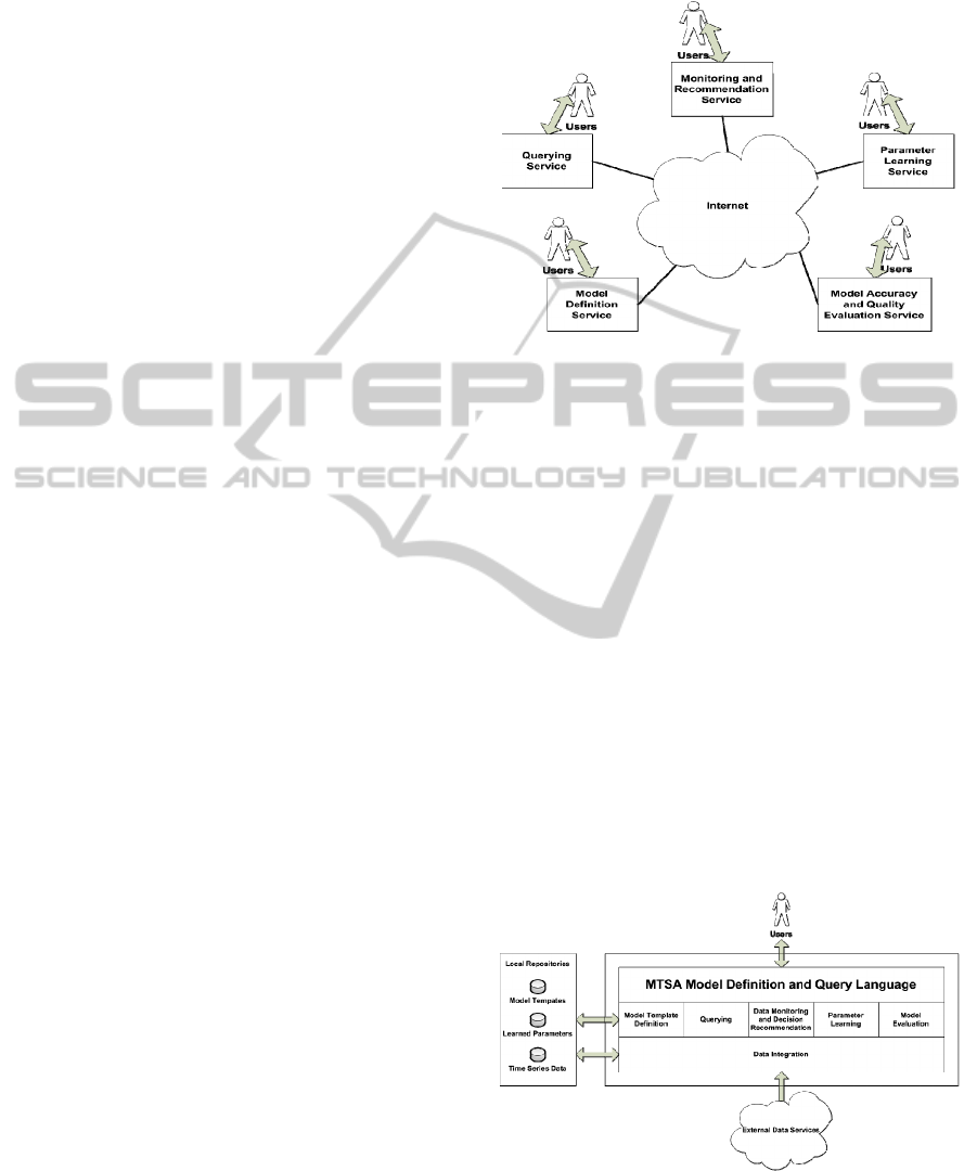
Figure 1 shows a range of common services that is
desirable to be offered over the internet. The MTSA
Model Definition Service provides a parametric
model template identified by the domain experts. In
the financial example that predicts the market
bottom, the model template may consist of indices
such as S&P 500 percentage decline (SPD),
Coppock Guide (CG), etc. These indices are
associated with their respective inequality
constraints, for example, SPD < p
1
, and CG < p
2
.
Given such a parametric model template in a given
domain, the Monitoring and Recommendation
Service continuously screens the incoming data
stream for indices that satisfy all the constraints
which specify when the event of interest, e.g., the
market bottom, has occurred, and recommends an
action, e.g., buying stock. Note that in the traditional
approach, the decision parameters p
1
and p
2
are
specified by the domain experts, e.g., SPD < -20%,
and CG < 0. However, using hard-set parameters
cannot capture the dynamics of the rapidly changing
market. The Parameter Learning Service
parameterizes the template, e.g., SPD < p
1
and CG <
p
2
, and supports learning of the parameters from the
historic time series. The accuracy of the decision
parameters are ensured through the Model Accuracy
and Quality Evaluation Service, which validates the
prediction, i.e., market bottom, with the observed
real data, and updates the model if necessary. The
Querying Service allows the service developers and
database programmers to express the complex
information services over multivariate time series
mentioned above in a high-level abstraction.
The service framework for multivariate time
series analytics (MTSA) provides a medium that
supports quick implementation of the services
described above. The MTSA service framework is
illustrated in Figure 2.
Figure 1: Services for Multivariate Time Series Over
Internet.
It consists of three layers: data integration,
information processing, and query language. The top
layer is the MTSA Model Definition and Query
Language, which extends the relational model with
time series and SQL with MTSA constructs. The
middle layer supports the MTSA constructs
including MTSA model template definition,
querying, parameter learning, model evaluation, data
monitoring, and decision recommendation. The
bottom, Data Integration Layer, allows service
providers to interact with external data services and
collect time series data from heterogeneous sources,
as well as from local repositories. This integration
layer provides a concentric view of the collected
data. The integration of the model template and the
learned parameters, which may be available both
locally and through external services, is also
supported by the Data Integration Layer.
Figure 2: A Service Framework for Multivariate Time
Series Analytics.
ICEIS 2011 - 13th International Conference on Enterprise Information Systems
94

3 EXPERT QUERY
PARAMETRIC ESTIMATION
(EQPE) MODEL
In this section, we discuss in detail the
methodologies used in the Parameter Learning
Service and the Monitoring and Recommendation
Service in the MTSA framework. More specifically,
we review the mathematical formulations of the
Expert Query Parametric Estimation (EQPE)
problem and solution. We also use the examples to
explain them in detail.
The goal of an EQPE problem is to find optimal
values of decision parameters that maximize an
objective function over historical, multivariate time
series. For an EQPE problem being constructed, we
need to define a set of mathematical notations and a
model for it. We assume that the time domain T is
represented by a set of natural numbers: T = N, and
that we are also given a vector of n real-valued
parameter variables (p
1
, p
2
, …, p
n
).
Definition 1. Time Series: A time series S is a
function S: T → R, where T is the time domain, and
R is the set of real numbers.
Definition 2. Parametric Monitoring Constraint: A
parametric monitoring constraint C(S
1
(t), S
2
(t), …,
S
k
(t), p
1
, p
2
, …, p
n
) is a symbolic expression in terms
of S
1
(t), S
2
(t), …, S
k
(t), p
1
, p
2
, …, p
n
, where S
1
(t),
S
2
(t), …, S
k
(t) are time series, t ∈ T is a time point,
and (p
1
, p
2
, …, p
n
) is a vector of parameters.
We assume a constraint C written in a language
that has the truth-value interpretation I: R
k
x R
n
→
{True, False}, i.e., I(C(S
1
(t), S
2
(t), …, S
k
(t), p
1
, p
2
,
…, p
n
)) = True if and only if the constraint C is
satisfied at the time point t ∈ T and with the
parameters (p
1
, p
2
, …, p
n
) ∈ R
n
. In this paper, we
focus on conjunctions of inequality constraints:
C(S
1
(t), S
2
(t), …, S
k
(t), p
1
, p
2
, …, p
n
) = ∧
i
(S
i
(t) op
p
j
), where op ∈ {<, ≤, =, ≥, >}.
Definition 3. Time Utility Function: A time utility
function U is a function U: T → R.
Definition 4. Objective Function: Given a time
utility function U: T → R and a parametric
constraint C, an objective function O is a function O:
R
n
→ R, which maps a vector of n parameters on R
n
to a real value R, defined as follows. For (p
1
, p
2
, …,
p
n
) ∈ R
n
, O(p
1
, p
2
, …, p
n
) ≝ U(t), where U is the
utility function, and t ∈ T is the earliest time point
that satisfies C, i.e.,
(1) S
1
(t) op
1
p
1
∧ S
2
(t) op
2
p
2
∧ … ∧ S
n
(t) op
n
p
n
is satisfied, and
(2) There does not exist 0 ≤ t' < t, such that S
1
(t')
op
1
p
1
∧ S
2
(t') op
2
p
2
∧ … ∧ S
n
(t') op
n
p
n
is satisfied.
Definition 5. Expert Query Parametric Estimation
(EQPE) Problem: An EQPE problem is a tuple <S,
P, C, U>, where S = {S
1
, S
2
, …, S
k
} is a set of k time
series, P = {p
1
, p
2
, …, p
n
} is a set of n real-value
parameter variables, C is a parametric constraint in S
and P, and U is a time utility function.
Intuitively, a solution to an EQPE problem is an
instantiation of values into the vector P of n real-
value parameters that maximizes the objective O.
Definition 6. Expert Query Parametric Estimation
(EQPE) Solution: A solution to the EQPE problem
<S, P, C, U> is argmax O(p
1
, p
2
, …, p
n
), i.e., the
(estimated) values of parameters, p
1
, p
2
, …, p
n
, that
maximize O, where O is the objective function
corresponding to U.
The base time series in our financial example are
shown in Table 1. We suppose that the first starting
date in any time-series data set is t = 0. Note that
some base time series are the direct inputs, whereas
some are used to derive another set of time series.
For instance, the derived time series in our case
study are shown in Table 2. The decision parameters
used in the case study are defined in Table 3. Let us
consider the following constraint C as an
illustration:
C(SPD(t), CG(t), CCD(t), ISM(t), NLCD(t), p
1
,
p
2
, p
3
, p
4
, p
5
) = SPD(t) < p
1
∧ CG(t) < p
2
∧
CCD(t) < p
3
∧ ISM(t) < p
4
∧ NLCD(t) > p
5
It means that the parametric monitoring
constraint C is satisfied, i.e., its interpretation is
True, if the above inequalities with the decision
parameters are satisfied at the time point t. The
interpretation also indicates that the monitoring
event occurs. We assume that the investor buys the
S&P 500 index fund at the decision variable time t
and sell it at the given t
S
, which is the last day of the
given training data set. The earning function SP(t
S
)/
SP(t) – 1 ∈ R is the utility, which is maximized by
choosing the optimal value t ∈ T, where SP(t
S
) and
SP(t) are the sell and buy value of the S&P 500
index fund at the time t
S
and t respectively. The
EQPE problem and solution for our example can be
constructed by putting the considered time series,
parameters, constraints, and functions to the
definitions shown in Table 4.
Table 1: Base Time-Series Data.
Base Time Series S Abbreviation
S&P 500 SP500(t)
Coppock Guide CG(t)
Consumer Confidence CC(t)
ISM Manufacturing Survey ISM(t)
Negative Leadership Composite NLC(t)
A SERVICE FRAMEWORK FOR LEARNING, QUERYING AND MONITORING MULTIVARIATE TIME SERIES
95

Table 2: Derived Time-Series Data.
Derived Time Series S Abbreviation
Percentage decline in SP(t) at the time
point t
SPD(t)
Points drop in CC(t) at the time point t CCD(t)
Number of consecutive days in Bear
Market “DISTRIBUTIOIN” of NLC(t)
at and before the time point t
NLCD(t)
Time Utility Earning at the time point t,
i.e., the index fund is bought at t and
sold at t
s
, where t
s
is the last day of the
learning data set
Earning(t)
Table 3: Decision Parameters.
Parameter Interpretation
p
1
Test if SPD(t) is less than p
1
at t.
p
2
Test if CG(t) is less than p
2
at t.
p
3
Test if CCD(t) is less than p
3
at t.
p
4
Test if ISM(t) is less than p
4
at t.
p
5
Test if NLCD(t) is greater than p
5
at t.
Table 4: EQPE Problem and Solution Formulation for
S&P 500 Index Fund.
Problem and Solution
Problem:
<S, P, C, U>, where
S = {SPD, CG, CCD, ISM, NLCD}
P = {p
1
, p
2
, p
3
, p
4
, p
5
}
C = SPD(t) < p
1
∧ CG(t) < p
2
∧ CCD(t) < p
3
∧
ISM(t) < p
4
∧ NLCD(t) > p
5
U = SP(t
s
)/SP(t) - 1
Solution:
argmax O(p
1
, p
2
, p
3
, p
4
, p
5
) ≝ U(t)
The values of the optimal decision parameters
can be determined by using the learning algorithm,
Checkpoint. Before explaining the Checkpoint
algorithm in detail, we first review the concept of
Dominance.
Definition 7. Dominance ≻: Given an EQPE
problem <S, P, C, U> and any two time points t, t' ∈
T, we say that t' dominates t, denoted by t' ≻ t, if the
following conditions are satisfied:
(1) 0 ≤ t' < t, and
(2) ∀(p
1
, p
2
, …, p
n
) ∈ R
n
, C(S
1
(t), S
2
(t), …, S
k
(t),
p
1
, p
2
, …, p
n
) → C(S
1
(t'), S
2
(t'), …, S
k
(t'), p
1
, p
2
, …,
p
n
).
Intuitively, t' dominates t if for any selection of
parametric values, the query constraint satisfaction
at t implies the satisfaction at t'. Clearly, the
dominated time points should be discarded when the
optimal time point is being determined. We formally
claim that:
Claim 1 - Given the conjunctions of inequality
constraints, S
1
(t) op
1
p
1
∧ S
2
(t) op
2
p
2
∧ … ∧ S
k
(t) op
k
p
k
and the two time points t', t such that 0 ≤ t' < t, t'
≻ t if and only if S
1
(t') op
1
S
1
(t) ∧ S
2
(t') op
2
S
2
(t) ∧ …
∧ S
k
(t') op
k
S
k
(t). The proof is shown in Appendix.
For example, suppose there are three time series
S
1
, S
2
, S
3
and three decision parameters p
1
, p
2
, p
3
.
And the constraints are C(S
1
(t), S
2
(t), S
3
(t), p
1,
p
2
, p
3
)
= S
1
(t) ≥ p
1
∧ S
2
(t) ≥ p
2
∧ S
3
(t) ≤ p
3
. Also assume the
values for S
1
, S
2
, and S
3
at the time point t
1
, t
2
, and t
3
respectively in Table 5 shown in the next page.
In this case, the time point t
3
is dominated
because there is a time point t
1
that make the
inequality, S
1
(t
1
) ≥ S
1
(t
3
) ∧ S
2
(t
1
) ≥ S
2
(t
3
) ∧ S
3
(t
1
) ≤
S
3
(t
3
), equal to true.
On the contrary, for all t' < t, if S
1
(t') ¬op
1
S
1
(t) ∨
S
2
(t') ¬op
2
S
2
(t) ∨…∨ S
n
(t') ¬op
n
S
n
(t) is satisfied, t is
not dominated
by t' denoted by t' ⊁ t. Let us
consider the same example above. Because S
1
(t
1
) <
S
1
(t
2
) ∨ S
3
(t
1
) > S
3
(t
2
), t
2
is not dominated.
4 CHECKPOINT ALGORITHM
AND EXPERIMENTAL
EVALUATION
Conceptually, we can search a particular set of
parameters {p
1
, p
2
, …, p
n
} which is at the earliest
time point t that is not dominated by any t' such that
the value of the objective function O is maximal
among all the instantiations of values into
parameters. However, the problem of this approach
is that for every single parameter set at t in a
learning data set, the parameter set at t has to be
examined with all the previous sets of parameters at
t' for checking the non-dominance before the
optimal solution can be found. In fact, due to the
quadratic nature, the conceptual approach is time
consuming and expensive particularly if the size of
the learning data set is significantly large. Instead,
the Checkpoint algorithm uses the KD-tree data
structure and searching algorithm to evaluate
whether a time point t is dominated based on the
Claim 1 for checking the non-dominance. The
pseudo code of the algorithm is:
Input: <S, P, C, U>
Output: p[1…k] is an array of the
optimal parameters that maximize
the objective.
Data Structures:
1. N is the size of the learning data
set.
ICEIS 2011 - 13th International Conference on Enterprise Information Systems
96

2. T
kd
is a KD tree that stores the
parameter vectors that are not
dominated so far.
3. MaxT is the time point that gives
the maximal U so far, denoted by MaxU.
Processing:
STEP 1: T
kd
:= <S
1
(0), S
2
(0), …,
S
k
(0)>;
MaxT := 0;
MaxU := U(0);
STEP 2: FOR t := 1 TO N - 1 DO {
Non-Dominance Test: Query the T
kd
to find if there exists a point
(
1
, 
2
, …, 
k
) in the T
kd
, which
is in the range [S
1
(t), ∞) x
[S
2
(t), ∞) x … x [S
k
(t), ∞).
IF (NOT AND t is not dominated
AND U(t) > MaxU) THEN Add
<S
1
(t), S
2
(t), …, S
k
(t)> to T
kd
;
MaxT := t;
MaxU := U(t);}
STEP 3: FOR i := 1 TO k DO {
p[i] := S
i
(MaxT);}
STEP 4: RETURN p[1…k];
Clearly, the first time point is not dominated
because there is no time point preceding it.
Therefore, <S
1
(0), S
2
(0), …, S
k
(0)> can be added to
T
kd
. 0 and U(0) can be assigned to MaxT and MaxU
respectively.
Using the Checkpoint algorithm step by step for
the problem shown in Table 5, we can search
through a particular set of parameters {p
1
, p
2
, p
3
}
which is at the earliest time point t that is not
dominated by any t' such that the value of the utility
function U is maximal. In STEP 1, the <S
1
(t
1
),
S
2
(t
1
), S
3
(t
1
)> is added to the T
kd
since it is the first
time point. Then t
1
and U(t
1
) are assigned to MaxT
and MaxU respectively. In STEP 2, t
2
is not
dominated because S
1
(t
1
) < S
1
(t
2
) ∧ S
2
(t
1
) > S
2
(t
2
) ∧
S
3
(t
1
) > S
3
(t
2
) does not satisfy the Claim 1. However,
t
3
is dominated because S
1
(t
1
) > S
1
(t
3
) ∧ S
2
(t
1
) > S
2
(t
3
)
∧ S
3
(t
1
) < S
3
(t
3
) does satisfy the Claim 1. <S
1
(t
2
),
S
2
(t
2
), S
3
(t
2
)> is added to the T
kd
because t
2
is not
dominated and U(t
2
) > U(t
1
). Thus t
2
and U(t
2
) are
assigned to MaxT and MaxU respectively. In STEP
3, p[1] := S
1
(MaxT), p[2] := S
2
(MaxT), and p[3] :=
S
3
(MaxT) in the for-loop statement. In STEP 4, the
algorithm returns 25, 15, and 2.
The time complexity for the range search and
insertion of a parameter vector in the T
kd
tree is
O(klogN) respectively.
Theorem 1: For N parameter vectors in the data set,
the Checkpoint algorithm correctly computes an
EQPE solution, i.e., argmax O(p
1
, p
2
, p
3
, p
4
, p
5
),
where O is the objective function of the EQPE
problem, with the complexity O(kNlogN). The proof
of the theorem is shown in Appendix.
Using the Checkpoint algorithm, we can obtain
the optimal decision parameters and the maximal
earning from the training data set for the financial
problem shown in Table 6. The time complexity of
the MLE for the logit regression model is O(k
2
N),
where k is the number of decision parameters, and N
is the size of the learning data set. For the
Checkpoint algorithm, the complexity is O(kNlogN).
Using the decision parameters from the financial
expert (i.e., -20%, 0, -30, 45, 180 days), the logit
regression model, and the Checkpoint algorithm, the
“Best Buy” opportunities in stock and their earnings
are shown in Table 7. Note that the Checkpoint
algorithm considerably outperforms both the
financial expert’s criteria and the logit regression
model.
Table 5: Values of S
1
, S
2
, S
3
, and U at the time point t
1
, t
2
,
and t
3
.
Time S
1
S
2
S
3
U
t
1
13 27 3 10
t
2
25 15 2 200
t
3
10 20 5 150
Table 6: Optimal Decision Parameters and Maximum
Earning (%) from the Learning Data Set
1
.
p
1
p
2
p
3
p
4
p
5
O(p
1
,p
2
,p
3
,p
4
,p
5
)
-29.02
-
20.01
-
26.61
49 70 53.37
Table 7: Investors’ Earning of the S&P 500 Index Fund
from the Test Data Set
2
.
Decision
Approach
Best
Buy
S&P
500 Index
Earning
%
Financial Expert’s
Criteria
10/09/08 909.92 1.03
Logit Regression
Model
11/26/08 887.68 3.56
Checkpoint
Algorithm with
Financial Expert’s
Template
03/10/09 719.6 27.8
1. The learning data set is from 06/01/1997 to 06/30/2005.
2. The test data set is from 07/01/2005 to 06/30/2009 that is the
sell date of the fund with the value of 919.32.
A SERVICE FRAMEWORK FOR LEARNING, QUERYING AND MONITORING MULTIVARIATE TIME SERIES
97

5 MTSA DATA MODEL
AND QUERY LANGUAGE
5.1 Data Model
The time-series (TS) data model is an extension of
the relational model with specialized schemas. A
time-series schema is of the form TSname(T:Time,
Vname:Vtype), where Time and Vtype are data
types, Vtype is either Real or Integer, and TSname
and Vname are names chosen by users.
A time-event (TE) schema is of the form
TEname(T:Time, Ename:Binary), where Binary is
the binary type corresponding to the domain {0,1},
and TEname and Ename are names chosen by users.
A TS database schema is a set of relational
schemas which may include (specific) TS and/or TE
schemas.
A TS tuple over a schema TSname(T:Time,
Vname:Vtype) is a relational tuple over that schema,
i.e., a mapping m: {T, Vname} → Dom(Time) x
Dom(Vtype), such that m(T) ∈ Dom(Time) and
m(Vname) ∈ Dom(Vtype).
A TE tuple over a similar schema
TEname(T:Time, Ename:Binary) is a mapping m:
{T, Ename} → Dom(Time) x Dom(Binary), such
that m(T) ∈ Dom(Time) and m(Ename) ∈
Dom(Binary).
Let us consider our financial example. In the
market-bottom scenario, the service provider can use
the querying service to create the base, derived, and
related time-series tables as inputs and store them in
the database. The base time-series tables are
SP500(T, Index), CG(T, Index), CC(T, Index),
ISM(T, Index), and NLC(T, Index).
5.2 Querying Service
Using the base time series tables, we can generate
derived time series tables (if any) by the traditional
SQLs. In our case study, some derived time series
tables, e.g., SPD(t), CCD(t), etc., are:
CREATE VIEW SPD AS (
SELECT After.T, After.Average /
Before.Average – 1 AS Value
FROM (SELECT SP1.T,AVG(SP2.Index)
AS Average
FROM SP500 SP1, SP500 SP2
WHERE SP2.T <= SP1.T
AND SP2.T >= SP1.T – 6
AND SP1.T – 6 >= 0
GROUP BY SP1.T) After,
(SELECT SP1.T, AVG(SP2.Index) AS
Average
FROM SP500 SP1, SP500 SP2
WHERE SP2.T <= SP1.T – 150
AND SP2.T >= SP1.T – 156
AND SP1.T – 156 >= 0
GROUP BY SP1.T) Before
WHERE After.T = Before.T);
CREATE VIEW CCD AS (
SELECT After.T, (After.Average –
Before.Average) AS Value
FROM (SELECT CC1.T,AVG(CC2.Index)
AS Average
FROM CC CC1, CC CC2
WHERE CC2.T <= CC1.T
AND CC2.T >= CC1.T – 6
AND CC1.T – 6 >= 0
GROUP BY CC1.T) After,
(SELECT CC1.T,AVG(CC2.Index)
AS Average
FROM CC CC1, CC CC2
WHERE CC2.T <= CC1.T – 150
AND CC2.T >= CC1.T – 156
AND CC1.T – 156 >= 0
GROUP BY CC1.T) Before
WHERE After.T = Before.T);
5.3 Monitoring and Recommendation
Service
Using the monitoring and recommendation service
over the new incoming data, the financial analyst
can recommend the investors whether or not they
should buy the stock. In our example, the input
parametric time series tables for monitoring are
SPD(T, Value), CG(T, Index), CCD(T, Value),
ISM(T, Index), and NLCD(T, Value). The
monitoring and recommendation service can be
expressed by a monitoring view and executed by the
MONITOR command.
CREATE VIEW MarketBottomTable AS (
SELECT SPD.T,(CASE WHEN SPD.Value <
PR.p
1
AND CG.Index < PR.p
2
AND CCD.Value < PR.p
3
AND
ISM.Index < PR.p
4
AND
NLCD.Value > PR.p
5
THEN ‘1’
ELSE ‘0’ END) AS MB
FROM SPD, CG, CCD, ISM, NLCD,
Para PR
WHERE SPD.T = CG.T AND CG.T =
CCD.T AND CCD.T = ISM.T AND ISM.T =
NLCD.T);
CREATE VIEW
MB_Monitoring_Recommendation
AS (SELECT MBT.T, (CASE WHEN MBT.MB
= ‘1’ THEN ‘Market
Bottom Is Detected.
Buy Stock Is
Recommended.’
END) AS Action
FROM MarketBottomTable MBT);
MONITOR MB_Monitoring_Recommendation;
ICEIS 2011 - 13th International Conference on Enterprise Information Systems
98

where Para is a table to store the decision
parameters, e.g., p
1
= -20, p
2
= 0, p
3
= -30, p
4
= 45,
and p
5
= 180. If the parametric monitoring constraint
in the CASE WHEN clause is satisfied at the current
time point t, the value of the attribute “MB”
dedicates “1”. The service then recommends the
financial analysts to buy the index fund for the
investors since the market bottom is predicted.
5.4 Parameter Learning Service
As we discussed, the expert’s suggested parameters
(-20. 0, -30, 45, 180) are not accurate enough to
monitor the dynamic financial market at all time;
thus, the parameter learning service should be
adopted by expressing as follows:
Step 1: Store base TS tables, e.g.,
SP500, CG, CC, ISM, and NLC, in
the database.
Step 2: Define SQL views for derived
TS tables, e.g, SPD, CCD,
etc., shown in Section 5.2.
Step 3: Create a parameter table
which stores the optimal
decision parameters.
CREATE VIEW Para (
p
1
REAL,
p
2
REAL,
p
3
REAL,
p
4
REAL,
p
5
REAL);
Step 4: Create a TS view for the
time utility.
CREATE VIEW Earning AS (SELECT
SP1.T,
((Last.Index/SP1.Index –
1) * 100) AS Percent FROM SP500
SP1,
(SELECT SP2.Index
FROM SP500 SP2
WHERE SP2.T >= ALL
(SELECT SP3.T
FROM SP500 SP3)) Last);
Step 5: Create a learning event and
then execute the event
construct to learn the
parameters.
CREATE EVENT
LearnMarketBottomParameter (
LEARN Para PR
FOR MAXIMIZE E.Percent
WITH SPD.Value < PR.p
1
AND
CG.Index < PR.p
2
AND
CCD.Value < PR.p
3
AND
ISM.Index < PR.p
4
AND
NLCD.Value > PR.p
5
FROM SPD, CG, CCD, ISM,
NLCD, Earning E
WHERE SPD.T = CG.T AND
CG.T = CCD.T AND CCD.T =
ISM.T AND ISM.T = NLCD.T
AND NLCD.T = E.T;)
EXECUTE
LearnMarketBottomParameter;
When the event “LearnMarketBottomParameter”
is executed, the command “LEARN” will call for the
Checkpoint algorithm to solve the corresponding
EQPE problem and will put its solution in the Para
table, where all parameters, e.g., p
1
, p
2
, p
3
, p
4
, and p
5
are instantiated with optimal values.
6 CONCLUSIONS AND FUTURE
WORK
To the best of our knowledge, this is the first paper
to propose a service framework for multivariate time
series analytics that provides model definition,
querying, parameter learning, model evaluation,
monitoring, and decision recommendation over
multivariate time series data. The parameter learning
services combine the strengths of both domain-
knowledge-based and formal-learning-based
approaches for maximizing utility over multivariate
time series. It includes a mathematical model and a
learning algorithm for solving Expert Query
Parametric Estimation problems. Using the
framework, we conduct a preliminary experiment in
the financial domain to demonstrate that our model
and algorithm are more effective and produce results
that are superior to the two approaches mentioned
above. We also develop MTSA data model and
query language for the services of querying,
monitoring, and parameter learning. There are still
many open research questions, for example, what
models can capture different types of events and
how those events impact the services that the
framework provides.
REFERENCES
Bellman, R., 1961. Adaptive Control Processes: A Guided
Tour. Princeton, University Press.
Bentley, J. L., 1975. Multidimensional Binary Search
Trees Used for Associative Searching.
Communications of the ACM, Vol 18 Issue 09, p.
509-517, 1975.
A SERVICE FRAMEWORK FOR LEARNING, QUERYING AND MONITORING MULTIVARIATE TIME SERIES
99

Bentley, J. L., 1979. Multidimensional Binary Search
Trees in Database Applications, Vol 5 Issue 04, p.
333-340. IEEE Transactions on Software Engineering.
Brodsky, A., Henshaw, S.M., and Whittle, J., 2008.
CARD: A Decision-Guidance Framework and
Application for Recommending Composite
Alternatives. 2
nd
ACM International Conference on
Recommender Systems.
Brodsky, A. and Wang. X. S., 2008. Decision-Guidance
Management Systems (DGMS): Seamless Integration
of Data Acquisition, Learning, Prediction, and
Optimization. Proceedings of the 41st Hawaii
International Conference on System Sciences.
Brodsky, A., Bhot, M. M., Chandrashekar, M., Egge, N.E.,
and Wang, X.S., 2009. A Decisions Query Language
(DQL): High-Level Abstraction for Mathematical
Programming over Databases. Proceedings of the
35th SIGMOD International Conference on
Management of Data.
Dougherty, C., 2007. Introduction to Econometrics (Third
Edition). Oxford University Press.
Dumas, M., O’Sullivan, J., Heravizadeh, M., Edmond, D.,
and Hofstede, A., 2001. Towards a Semantic
Framework for Service Description. Proceedings of
the IFIP TC2/WG2.6 Ninth Working Conference on
Database Semantics: Semantic Issues in E-Commerce
Systems.
Erl, T., 2005. Service-Oriented Architecture (SOA):
Concepts, Technology, and Design. Prentice Hall.
Erradi, A., Anand, S., and Kulkarni, N., 2006. SOAF: An
Architectural Framework for Service Definition and
Realization. IEEE International Conference on
Services Computing (SCC'06).
Hansen, B. E., 2010. Econometrics. University of
Wisconsin. http://www.ssc.wisc.edu/~bhansen/
econometrics/Econometrics.pdf.
Harrington, J., 2009. Relational Database Design and
Implementation (Third Edition). Morgan Kaufmann.
Heij, D., De Boer, P., Franses, P. H., Kloek, T., and Van
Dijk, H. K., 2004. Econometric Methods with
Applications in Business and Economics. Oxford
University Press.
Holyfield, S., 2005. Non-technical Guide to Technical
Frameworks. JISC CETIS.
http://www.elearning.ac.uk/features/nontechguide1.
Josuttis, N., 2007. SOA in Practice: The Art of Distributed
System Design. O'Reilly Media.
Ngan, C. K., Brodsky, A., and Lin, J., 2010. Decisions on
Multivariate Time Series: Combining Domain
Knowledge with Utility Maximization. The 15th IFIP
WG8.3 International Conference on Decision Support
Systems.
Nicholls, P., 2009. Enterprise Architectures and the
International e-Framework. e-framework
Organization. http://www.e-
framework.org/Portals/9/docs/EAPaper_2009-07.pdf
Olivier, B., Roberts, T., and Blinco, K., 2005. The e-
Framework for Education and Research: An
Overview. e-framework Organization. http://www.e-
framework.org/Portals/9/Resources/eframeworkrV1.p
df.
Ort, Ed. Service-Oriented Architecture and Web Services:
Concepts, Technologies, and Tools. Sun Developer
Network Technical Articles and Tips.
http://java.sun.com/developer/technicalArticles/WebS
ervices/soa2/
Papazoglou, M., and Heuvel, W., 2005. Service Oriented
Architectures: Approaches, Technologies, and
Research Issues. The VLDB Journal, June.
Quartel, D., Steen, M., Pokraev S., and Sinderen, M.,
2007. COSMO: A Conceptual Framework for Service
Modelling and Refinement, Volume 9, Numbers 2-3,
225-244, July. Journal of Information Systems
Frontiers.
Ralph H. Sprague, Jr., 1980.
A Framework for the
Development of Decision Support Systems, Volume 4,
Number 4, 1-26, December. MIS Quarterly.
Samet, H., 2006. Foundations of Multidimensional and
Metric Data Structures. Morgan Kaufmann.
Stack, J. B., 2009. Technical and Monetary Investment
Analysis, Vol 9 Issue 3 & 5. InvesTech Research.
Stephen, B., et al., 2008. Database Design: Know It All.
Morgan Kaufmann.
Wilson, S., Blinco, K., and Rehak, D., 2004. Service-
Oriented Frameworks: Modelling the Infrastructure
for the Next Generation of e-Learning Systems. JISC
CETIS. http://www.jisc.ac.uk/uploaded_documents/
AltilabServiceOrientedFrameworks.pdf.
Zhang, T., Ying, S., and Cao, S., and Jia, S., 2006. A
Modeling Framework for Service-Oriented
Architecture. Proceedings of the Sixth International
Conference on Quality Software (QSIC'06).
ICEIS 2011 - 13th International Conference on Enterprise Information Systems
100

APPENDIX
Claim 1 - Given the conjunctions of inequality
constraints, S
1
(t) op
1
p
1
∧ S
2
(t) op
2
p
2
∧ … ∧ S
k
(t) op
k
p
k
and the two time points t', t such that 0 ≤ t' < t, t'
≻ t if and only if S
1
(t') op
1
S
1
(t) ∧ S
2
(t') op
2
S
2
(t) ∧ …
∧ S
k
(t') op
k
S
k
(t).
Proof:
Without loss of generality, we assume that op
i
=
“≤”, for all 1 ≤ i ≤ k. It is because “≥” can be
replaced with ≤ by changing a corresponding time
series S
i
(t) to - S
i
(t). For op
i
= “=”, we can use the
conjunction with both ≥ and ≤.
If Direction:
Assume that S
1
(t') ≤ S
1
(t) ∧ S
2
(t') ≤ S
2
(t) ∧ … ∧
S
k
(t') ≤ S
k
(t). For any (p
1
, p
2
, …, p
k
) ∈ R
k
and every i
= 1, 2, …, k, if S
1
(t) ≤ p
1
, then S
1
(t') ≤ p
1
because
S
1
(t') ≤ S
1
(t). Therefore, S
1
(t) ≤ p
1
∧ S
2
(t) ≤ p
2
∧ … ∧
S
k
(t) ≤ p
k
→ S
1
(t') ≤ p
1
∧ S
2
(t') ≤ p
2
∧ … ∧ S
k
(t') ≤ p
k
and then t' ≻ t.
Only If Direction:
Assume that t' ≻ t. Then S
1
(t) ≤ p
1
∧ S
2
(t) ≤ p
2
∧
… ∧ S
k
(t) ≤ p
k
→ S
1
(t') ≤ p
1
∧ S
2
(t') ≤ p
2
∧ … ∧ S
k
(t')
≤ p
k
. Therefore, for any (p
1
, p
2
, …, p
k
) ∈ R
k
and
every i = 1, 2, …, k, we have S
i
(t) ≤ p
i
→ S
i
(t') ≤ p
i
.
Proof of Theorem 1: The Checkpoint algorithm
correctly solves the EQPE problem, i.e., if argmax
O(p
1
, p
2
, p
3
, p
4
, p
5
), where O is the objective
function of the EQPE problem.
The time complexity is O(kNlogN), where k is
the number of time series and N is the size of the
learning data set.
Proof: To prove the correctness of the algorithm
if it is sufficient to show Claim 2: The Non-
Dominance test in STEP 2 of the Checkpoint
Algorithm is satisfied for the time point t if and only
if there does not exist t' that dominates t, where 0 ≤ t'
< t.
We prove it by induction on t, where 1 ≤ t ≤ N.
For t = 1, T
kd
= ∅ and t = 1 is not dominated;
therefore, the “if and only if” condition holds.
Assuming the correctness for 1, 2, …, t-1; it follows
the STEP 2 of the algorithm that T
kd
at point t
contains all non-dominated time points t', where t' ≤
t - 1.
If Direction:
The IF part of Claim 2 is straightforward since if
t is not dominated by an earlier time point t', such
point cannot appear on the T
kd
tree; therefore, the
Non-Dominance Test must be satisfied by Claim 1.
Only If Direction:
For the ONLY IF part of the Claim 2, assume
that the Non-Dominance test in STEP 2 of the
algorithm is satisfied. Then there does not exist the
time point t' on T
kd
for which (S
1
(t'), S
2
(t'), …, S
k
(t'))
∈ [S
1
(t), ∞) x [S
2
(t), ∞) x … x [S
k
(t), ∞), where 0 ≤ t'
< t. Assume that T
kd
at time t contains the time
points 


<


<⋯<


and assume, by
contradiction, that there exists t' that dominates t, t'
≻ t, where 0 ≤ t' < t. Clearly, t' is not one of



<


<⋯<


because they do not dominate t
by the induction hypothesis. Because t' was not
added to the T
kd
tree and the induction hypothesis,



≻
′
for some j = 1, 2, …, m. From the
contradiction assumption t' ≻ t and the transitivity of
≻, it follows that 


≻. Thus, by Claim 1,


(


)≤

() ∧ 

(


)≤

() ∧ ⋯ ∧ 

(


)≤


() which contradicts the fact that the Non-
dominance test in STEP 2 was satisfied for t. This
completes the proof of Claim 2 and of the
correctness of the algorithm.
Time Complexity: The algorithm performs N
iterations in STEP 2, spending time O(klogN) using
the T
kd
algorithm (Bentley, 1975 & 1979) for the T
kd
range query in Non-Dominance Test. Thus the
overall complexity is O(kNlogN).
A SERVICE FRAMEWORK FOR LEARNING, QUERYING AND MONITORING MULTIVARIATE TIME SERIES
101