
KEYWORDS EXTRACTION
Selecting Keywords in Natural Language Texts with Markov Chains
and Neural Networks
Bła
˙
zej Zyglarski and Piotr Bała
Faculty of Mathematics and Computer Science, Nicolaus Copernicus University, Chopina St. 13/18, Torun, Poland
Keywords:
Keywords extraction, Text mining, Neural networks, Kohonen, Markov chains.
Abstract:
In this paper we show our approach to keywords extraction by natural language processing. We present revised
and extended version of previously shown document analysis method, based on Khonen Neural Networks with
Reinforcement, which uses data from the large document repository to check and improve results. We describe
new improvements, which we’ve achieved with preprocessing set of words and creating initial ranking using
Markov Chains. Our method shows, that keywords can be selected from the text with great accuracy. In this
paper we present evaluation and comparison of both methods and example results of keywords selection upon
random documents.
1 INTRODUCTION
Large increase of available data can be noticed nowa-
days. Modern search engines use simple language
querying and return results containing query words.
Most of the results are unfortunatelyinadequate to the
question. It shows that very important modern com-
puter science problems is automatic analysis of data,
which is able to pinpoint most important parts of data.
Problem is easier, if the data is structurised and the
structure is known (e.g. specific databases). Chal-
lenge is to find the structure in "free language". We
have developed algorithms, which can analyse text
with use of structual distance between words and Ko-
honen Neural Networks with Reinforcement based on
previously computed distances between documents in
the large repository (see (Zyglarski and Bała, 2009)).
It means that effective keywords selection needs a
large knowledge about background information such
as other documents. This approach is similar to hu-
man learning, which can be more effective, if a per-
son knows more. In this article we introduce extended
version of this algorithm, imporooved by text prepro-
cessing and computing initial words weights (instead
of using 1 as startup weights) with use of Markov
Chains built on idea of PageRank.
2 NEURAL NETWORKS
CATEGORIZATION
ALGORITHM
Our idea of keywords selection used a distance be-
tween words defineded as:
Lets
b
T
f
=
b
T( f) be a text extracted from a docu-
ment f and
b
T
f
(i) be a word placed at the position i
in this text. Lets denote the distance between words A
and B within the text
b
T
f
as δ
f
(A,B).
δ
f
(A,B) = (1)
= min
i, j∈{1,..,n}
{ki− jk;A =
b
T
f
(i) ∧B =
b
T
f
( j)} (2)
By the position i we need to understand a number of
additional characters (such as space, dots and com-
mas) read so far during reading text. Every sentence
delimiter is treated like a certain amount W of white
characters in order to avoid combining words from
separate sequences. After tests we choose differend
W for different additional characters, as is shown in
table 1
The knowledge of distances between words in
document was used to categorize them with use of the
self-organizing Kohonen Neural Network (figure 1)
(Kohonen, 1998).
The categorization procedure consisted of 5 steps:
1. Create rectangular m ×m network, where m =
⌊
4
√
n⌋, where n is number of all words Presented
315
Zyglarski B. and Bała P..
KEYWORDS EXTRACTION - Selecting Keywords in Natural Language Texts with Markov Chains and Neural Networks.
DOI: 10.5220/0003088003150321
In Proceedings of the International Conference on Knowledge Management and Information Sharing (KMIS-2010), pages 315-321
ISBN: 978-989-8425-30-0
Copyright
c
2010 SCITEPRESS (Science and Technology Publications, Lda.)

Table 1: Weights of additional characters.
Character Weight Reason
":", 2 weak relation
";" 10 very weak relation
".!?" 30 no relation
" " and others 1 strong relation
Figure 1: The scheme of the neural network for words cat-
egorization with selected element and its neighbors.
algorithm can distinguish maximally m
2
cate-
gories. Every node (denoted as ω
x,y
) is con-
nected with four neighbors and contains a proto-
type word (denoted as
b
T
f
ω
(x,y)) and a set (denoted
as β
f
ω
(x,y)) of locally close words.
2. For each node choose random prototype of the
category p ∈ {1,2,...,n}.
3. For each word k ∈ {1,2,..., n} choose closest
prototype
b
T
f
ω
(x,y) in network and add it to list
β
f
ω
(x,y).
4. For each network node ω
x,y
compute a general-
ized median for words from β
f
ω
(x,y) and neigh-
bors lists (denoted as β). A generalized median is
defined as an element A which minimizes a func-
tion:
Σ
B∈β
δ
f2
(A,B) (3)
Set
b
T
f
ω
(x,y) = A
5. Update word weights, by checking if other docu-
ments containing actually best (highest positions
in result list) words are in fact related to analysed
one:
For random number of actually best words:
• check random number of documentscontaining
this word,
• if more than 66% is close enough to analyzed
one, increase weight of tested keyword,
• if less than 33% is close enough to analyzed
one, decrease weight of tested keyword;
6. Repeat, until the network is stable. Stability of the
network is achieved, when in two following itera-
tions all word lists are unchanged (without paying
attention to iternal lists sturcture and their position
in nodes).
Such algorithm divided the set of all words found in
document into separate subsets, which contained only
locally close words. In other words it groupped words
into related sets. During it’s workflow weight of each
keyword candidate was updated, by checking if this
word can be found in similar documents. Similarity
of documents was checked with use of three kinds of
distances:
Let’s S
x
=
∑
i=1..n
x
i
a S
y
=
∑
i=1..n
y
i
. Let’s de-
fine distance between documents P
1
(x
1
,x
2
,...,x
n
) and
P
2
(y
1
,y
2
,...,y
n
) as
d
s
((x
1
,x
2
,...,x
n
),(y
1
,y
2
,...,y
n
)) = (4)
|
x
1
S
x
−
y
1
S
y
|+ |
x
2
S
x
−
y
2
S
y
|+ ... + |
x
n
S
x
−
y
n
S
y
| (5)
where x
i
, y
i
mean number of occurences of word i id
document P
1
and P
2
.
Let’s define distance between documents
P
1
(x
1
,x
2
,...,x
n
) i P
2
(y
1
,y
2
,...,y
n
) as
d
n
((x
1
,x
2
,...,x
n
),(y
1
,y
2
,...,y
n
)) = (6)
|x
1
−y
1
|+ |x
2
−y
2
|+ ... + |x
n
−y
n
| (7)
where x
i
, y
i
mean number of occurences of n-gram i
ind document P
1
and P
2
.
Let’s define Kolmogorov distance between docu-
ments P
1
i P
2
as
d
k
(P
1
,P
2
) = (8)
K(P
1
|P
2
∗) −K(P
2
|P
1
∗)
K(P
1
,P
2
)
(9)
where K(−|−) is Conditional Kolmogorov Complex-
ity.
Document X is close to document Y if X is close
to Y in the meaning of d
s
, d
n
and d
k
.
Effectivenes of this method was quite good. Tests
show that in some examples correctness of results can
achieve even 90%, but in the most cases it is about
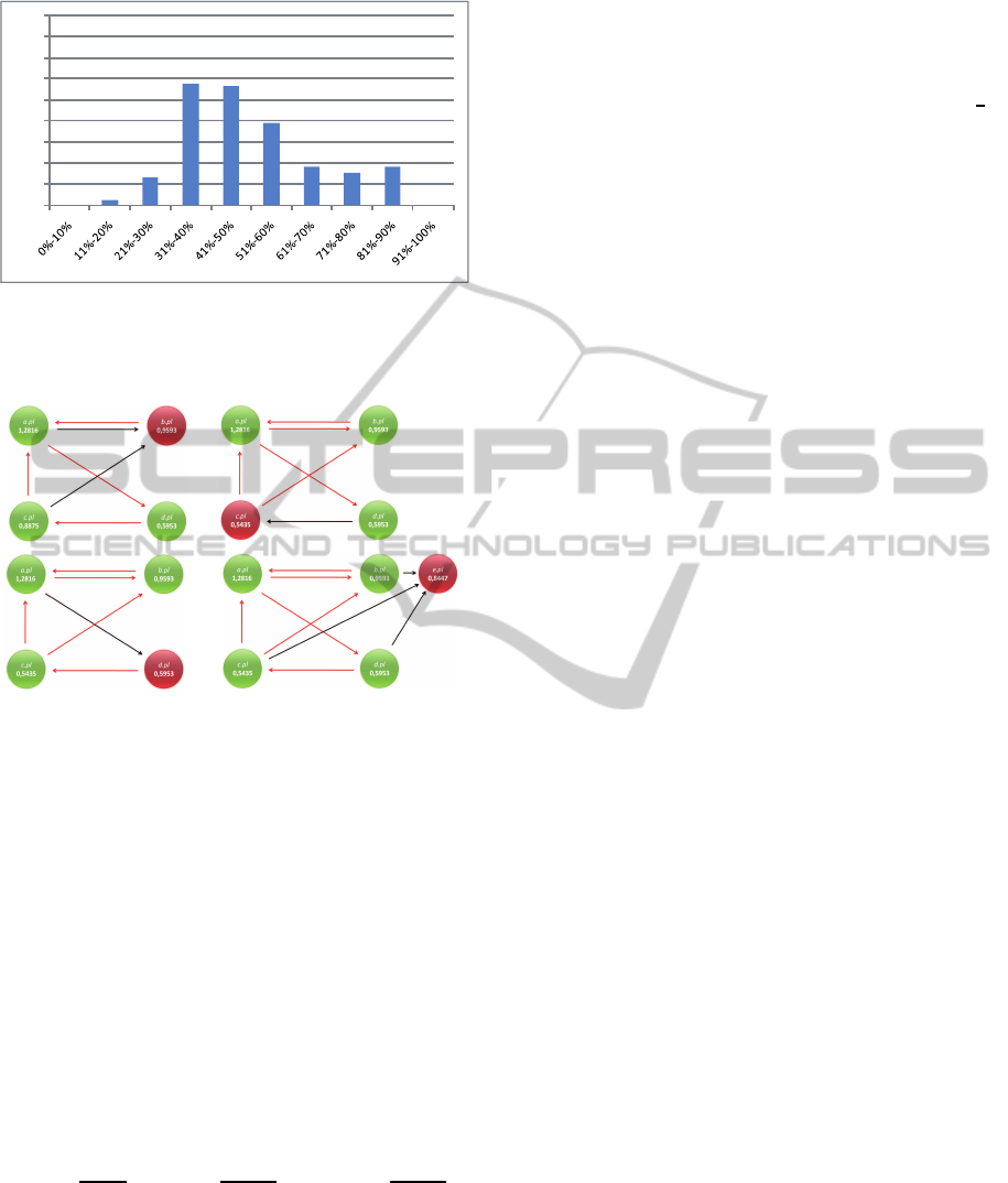
50%-70%. Results are shown on figure 2.
3 WEIGHTS PREPROCESSING
One of the assumption of this algorithm was equal
startup weights (= 1) of all words. We show, that
preprocessing this weight can signifitiantly improove
this results. This task can be performed with use of
Google PageRank idea ( (Avrachenkov and Litvak,
2004)).
KMIS 2010 - International Conference on Knowledge Management and Information Sharing
316
0%
5%
10%
15%
20%
25%
30%
35%
40%
45%
Figure 2: Effects of neural network method with reinforce-
ment. X axis shows effectiveness, Y axis shows number of
documents with processed with this effectiveness.
(a) (b)
(d)
(c)
Figure 3: Example PageRank computation.
3.1 PageRank
As states in (Avrachenkov and Litvak, 2004) PageR-
ank bases on knowledge about connections between
websites. Simply the site is as important, as impor-
tant are sites linking to it.
PageRank for every site depends on number of hy-
perlinks from other sites to considered one. Any hy-
perlink is interpreted as a vote.
Assuming that {X
1
,X
2
,...,X
n
} contain hyperlinks
pointing on page A, and kX
i
k means number of all
hyperlinks on page X
i
, kX
i
k
A
means number of hyper-
links pointing from X
i
to page A and PR
X
i
is PageR-
ank of X
i
page, and N is number of all websites in the
internet, then
PR
A
=
1−d
N
+ d(PR
X
1
kX
1
k
A
kX
1
k
+ ... + PR
X
n
kX
n
k
A
kX
n
k
)
PageRank algorithm constructs matrix P =
[p
ij
]
i, j∈N
, where p
ij
is a probability of moving from
page i to page j. Probability p
ij
equals quotient of
number of hyperlinks on page i pointing on page j
and number of all hyperlinks on page i, or 0 if there
are no hyperlinks from i and j. Then transition matrix
P
′
= cP + (1 −c)(1/n)E is defined, where E has all
elements equal to 1, and c is probability of concious
click on specific hyperlink. 1−c means random enter
to some page.
Algorithm assumes, that P(X
o
= s
i
) = p
i
(0) =
1
n
dla i = 1,..., n.
X
k
distribution is computed with:
[p
1
(k−1), p
2
(k−1),..., p
n
(k−1)]
p
′
11
p
′
12
... p
′
1n
p
′
21
p
′
22
... p
′
2n
.
.
.
.
.
.
.
.
.
p
′
n1
p
′
n2
... p
′
nn
= [p
1
(k), p
2
(k),..., p
n
(k)]
Sequence X
0
,X
1
,...,X
n
,... fulfill assumption for being
Markov Chain and P
′
is a transition matrix and (X
n
)
converges to stationary distribution π.
π(P
′
) = π
π1 = 1
3.2 Markov Chains
As states in (Bremaud, 2001) and (Haggstrom, 2002):
• a sequence of random variables (X
n
)
n=0,...
with
values in countable set S (state space) is called
Markov Chain when ∀
n∈N
and every sequence
s
0
,s
1
,...,s
n
∈ S
P(X
n
= s
n
|X
n−1
= s
n−1
,...,X
0
= s
0
) = (10)
P(X
n
= s
n
|X
n−1
= s
n−1
) (11)
if only P(X
n−1
= s
n−1
,...,X
0
= s
0
) > 0, it means
that state of chaing in time n (X
n
) depends only on
state in time n−1 (X
n−1
).
• Markov property: Matrix P = [p
ij
]
i, j∈S
is called
transition matrix on S, if all it’s elements are pos-
itive, and sum of elements in every row equals 1.
p
ij
≥ 0,
∑
k∈S
p
ik
= 1 (12)
• Random variable X
0
is called initial state and it’s
probability distribution v(i) = P(X
0
= i), is called
initial distribution.
• Distribution of the Markov Chain depends on ini-
tial distribution and transition matrix.
We’ve decided to use these Markov Chains to cre-
ate a startup ranking of words inside each document.
This ranking is used as input data for main Koho-
nen Neural Network algorithm. We’ve called it Wor-
dRank.
KEYWORDS EXTRACTION - Selecting Keywords in Natural Language Texts with Markov Chains and Neural Networks
317
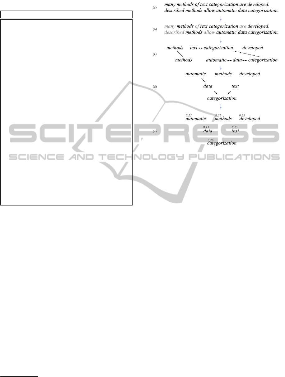
Table 2: Example keywords.
Example words connections
an ontology, ontology driven, driven similar-
ity, similarity algorithm, algorithm tech, tech
report, report kmi, kmi maria, maria var-
gas, vargas vera, vera and, and enrico, enrico
motta, motta an, an ontology, ontology driven,
driven similarity, driven similarity, similarity al-
gorithm, knowledge media, media institute, insti-
tute kmi, kmi the, the open, open university, uni-
versity walton, walton hall, hall milton, milton
keynes,keynes mk, mk aa, aa united, aa united,
united kingdom, kingdom m, m.vargas, vargas
vera , vera open, open.ac, ac.uk, uk abstract, ab-
stract.this, this paper, paper presents, presents our,
our similarity, similarity algorithm, algorithm be-
tween, between relations, relations in, in a, a user,
user query, query written, written in, in fol, fol
first, first order, order logic, logic and, and onto-
logical, ontological relations, relations.our, our
similarity, similarity algorithm, algorithm takes,
takes two, two graphs, graphs and, and produces,
produces a, a mapping, mapping between, be-
tween elements, elements of, of the, the two, two
graphs, graphs i.e, i.e.graphs, graphs associated,
graphs associated, associated to, to the, the query,
query a, a subsection, subsection of, of ontology,
ontology relevant
3.3 WordRank
While parsing simple text document, one have to find
relations between words. Our idea of Word Rank as-
sumes using of simple natural connections between
words, based on their position upon the text. Sim-
ply we can consider two words as connected, if they
are neighbours. Additionally, according to assump-
tions presented in previous papers, initial statistical
analysis of the texts in repository was performed and
unimportant words were chosen
1
. They should not be
considered during connections analysis and selection
connected words. Example set of connected words is
presented in table 2. All words, which are not om-
mited, are potential keywords.
Our procedure takes following steps, shown also
on figure 4.
1. Mark all punctuation marks and all unimportant
words as division elements. Mark all other words
as potential keywords. Lets V be a set of all po-
tential keywords.
1
Word is unimportant if it is appearing often in all ana-
lyzed documents.
Figure 4: Example graph of connected words
2. Set as connected every two neighbor words,
which are not marked as division elements. Con-
sider each connection as bidirectional.
3. Build directed graph G = (V,E).
4. Label every connection with weight from domain
[0,1]. (E = VxVx[0,1]) Let’s x and y be two
connected words. According to carried out tests,
weight of connection between word and its suc-
cessor should equal 1 and weight of connection
between word and its predecessor should equal
0.3.
E = E ∪{(x,y,1)}∪{(y,x,0.3)} (13)
5. For each word in graph compute it’s ranking ω() :
V → [0,2].
Now main algorithm of categorization presented
in (Zyglarski and Bała, 2009) can categorize those
words and prepare final keywords lists.
3.4 Main Part of the Algorithm
Last step of algorithm (For each word in graph com-
pute it’s ranking ω() : V → [0,2].) is the most im-
portant. It is based on the idea of Google PageR-
ank ((Page et al., 1999)), where importance of each
website depends on the number of hyperlinks, linking
to this website. Similarly in our algorithm, weight
of each word depends on weight and number of it’s
neighbors. By the word we need to understand ab-
stract class of the word (not connected with its posi-
tion in the text).
KMIS 2010 - International Conference on Knowledge Management and Information Sharing
318

Figure 5: Example workflow for preprocessing weights.
Weight ω(y) of word y in time t is calculated with
∀
y
ω
t
(y) =
p
n
+ (1− p)
∑
v∈V
ω(v,y) ∗ω
t−1
(v)
n
v
(14)
where n is number of words in the document, ω(v,w)
is the weight of the edge from v to w, and n
v
is a sum
of weights of all edges starting in v, and ω
0
(v) = 1.
p is a probability of fact, that analysed word is
keyword, while p −1 means that being keyword de-
pends on neighbor words.
While t → ∞, ω
t
(y) → ω(t). While repeating iter-
atively above equation, we can evaluate ω(t).
3.5 Theoretical Basis
This idea uses Markov Chains for creating Wor-
dRank.
Every step of above iteration can be represented in
matrix form.
Let’s P ∈M(n×n) = [p
ij
]
i, j=1,...,n
be a square ma-
trix, and n means number of words in the document.
Let’s p
ij
=
ω(i, j)
∑
k=1..n
ω(i,k)
, assuming, that p
ik
= 0 if word
i wasnt neighbor of j, and vice versa. Let’s W
i
be a
vector of weights of all words in text in time i. Let’s
W
0
=
¯
1.
Now we can define transition matrix P
′
= [p
′
ij
] ∈
M(n×n)
P
′
= p
1
n
1
1
.
.
.
1
+ (1− p)P
P
′
fullfill conditions of Markov property.
∑
j=1..n
p
ij
=
∑
j=1..n
ω(i, j)
∑
k=1..n
ω(i,k)
(15)
=
∑
j=1..n
ω(i, j)
∑
k=1..n
ω(i,k)
= 1 (16)
∑
j=1..n
p
′
ij
=
∑
j=1..n
p
1
n
+ (1− p)p
ij
(17)
=
∑
j=1..n
p
1
n
+
∑
j=1..n
(1− p)
ω(i, j)
∑
k=1..n
ω(i,k)
(18)
= p
∑
j=1..n
1
n
+ (1− p)
∑
j=1..n
ω(i, j)
∑
k=1..n
ω(i,k)
(19)
= p + (1 − p)
∑
j=1..n
p
ij
= p + 1 − p = 1 (20)
Let’s W
i
= P
′
W
i=1
. Let’s f : R
n
×M
n×n
(R) → R
n
.
Let’s (Z
k
) = P
′
∀
k∈N
and W
0
= E. Then chain W
i+1
=
f(W
i
,Z
i+1
) defines a Markov chain.
Proof is obvious.
Initial state of the chain is:
W
0
=
1
1
.
.
.
1
Then, each step of the algorithm is described by:
W
i
= P
′
W
i−1
and each state:
W
i
=
ω
i
(v
1
)
ω
i
(v
2
)
.
.
.
ω
i
(v
n
)
converges to stationary distribution W
′
, which
fullfills following:
W
′
= P
′
W
′
Proof of Convergence. We need to show, that W
′
exists and
W
′
= lim
n=0..∞
W
n
This proof needs a fundamental theorem of
Markov chains, prooved in (Grinstead and Snell,
1997).
Markov chain is called regular if all elements of
some power of transition matrix are ≥ 0.
KEYWORDS EXTRACTION - Selecting Keywords in Natural Language Texts with Markov Chains and Neural Networks
319
Theorem. Let’s P be the transition matrix of reg-
ular Markov chain. Sequence of P
i
converges with
i → ∞ to matrix M, which all rows are equal (den-
oded as m). Additionally m is a probability vector,
which means that it’s elements are ≥ 0 and their sum
equals 1.
Matrix P
′
defines regular Markov chain.
W
i
= P
′
W
i−1
= P
′i
W
0
Chain W
i
fullfills assumption of definition. Addi-
tioinally P
′n
converges to M. Any row m from matrix
M fullfils m = P
′
m. Let’s denote W
′
= m.
Theorem. Let’s P be the transition matrix of areg-
ular Markov chain and W = lim
n→∞
P
n
. Let’s w be a
row from W and c be a colum equal to
¯
1. Then
1. wP = w, and every vector v such as vP = v equals
w multiplied by a scalar,
2. Pc = c and every column x such as Px = x is a
column c multiplied by a scalar.
First proof of this theorem was described by Doe-
blin in (Doeblin, 1933).
This theorem proofs, that P
′n
W
0
→W
′
with n →
∞.
Convergence speed of P
′n
W
0
→W
′
is geomethri-
cal, so we can assume that W
′
equals W
k
for such k,
that |W
k
−W
k−1
| < ε for some small ε > 0
it means
|W
k
−W
k−1
| =
|ω
k
(v
1
) −ω
k−1
(v
1
)|
|ω
k
(v
2
) −ω
k−1
(v
2
)|
.
.
.
|ω
k
(v
n
) −ω
k−1
(v
2
)|
and
∀
s=1..n
|ω
k
(v
s
) −ω
k−1
(v
s
)| < ε
4 RESULTS DISCUSSION
Usage of this preprocessing of words weights signi-
ficiantly improoves efficiency of categorization algo-
rithm.
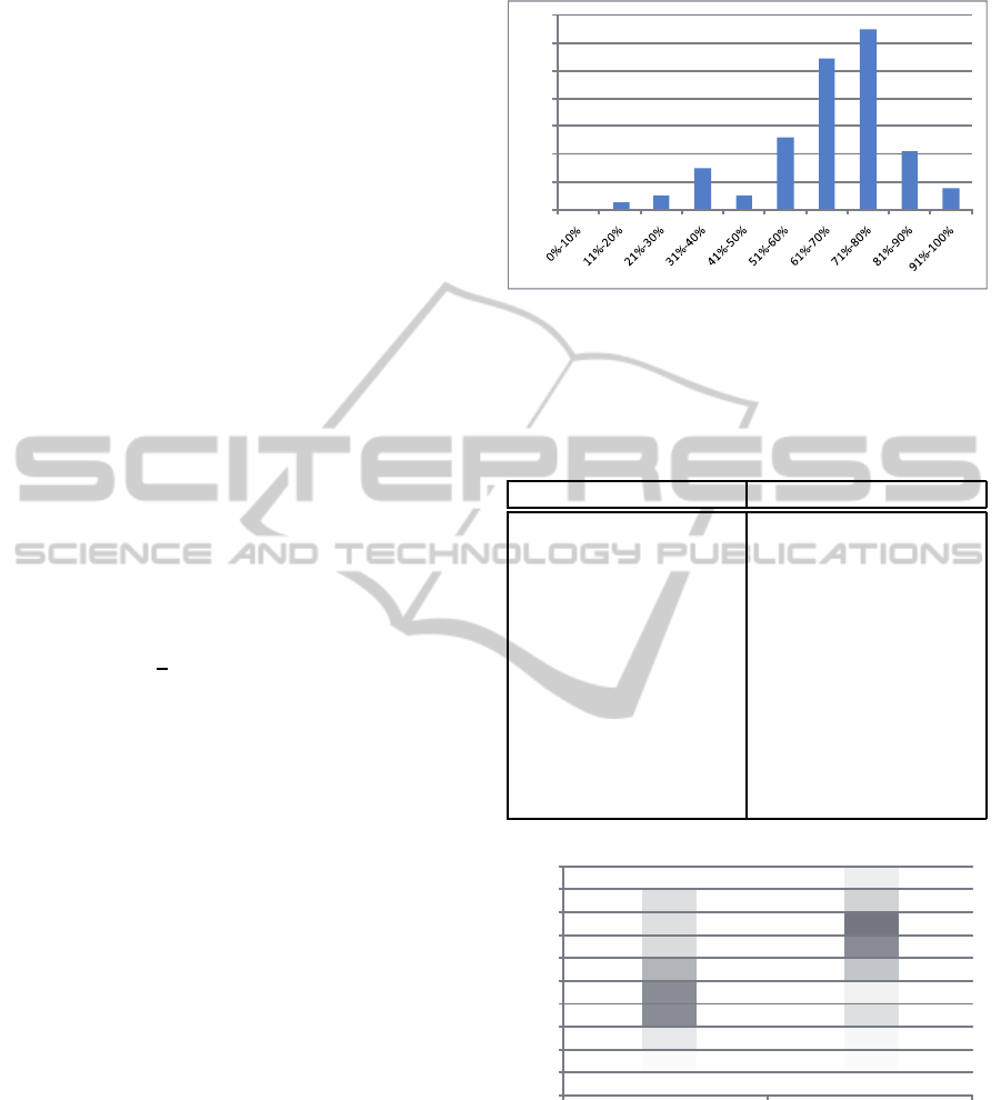
Table 3 shows example of keywords generated for
random document with and without usage of prepro-
cessing. Comparison of both methods tested on the
set of 1000 documents is presented on figure 7.
All results were checked empirically by reading
tested documents.
As it is shown on illustration 7 new algorithm can
produce more accurate results than the previous one.
In particular cases correctness of of keywords chose
can achieve even 100%, in most cases results are 80%
correct, which is great result.
0%
5%
10%
15%
20%
25%
30%
35%
Figure 6: Effects of neural network method with reinforce-
ment and preprocessing of the weights. X axis shows ef-
fectiveness, Y axis shows number of documents with pro-
cessed with this effectiveness.
Table 3: Example of keywords selection with and without
preprocessing.
without preprocessing with preprocessing
component , analyses,
deep , configuration ,
interface , described, ne
, generated , qa , lin-
guistic , names , stan-
dard , item , xsl , items
, extraction , grammar
, hpsg , np , id , named
, efficiency , evaluation
, lexical , attributes ,
semantics , elements ,
german , infl , main
parsing, german,
sentence, annotation,
id, architecture, xsl,
grammar, parser,
rmrs, linguistic, com-
ponent, pos, shallow,
nlp, whiteboard, deep,
string, hybrid, en,
structures, thesis
0%
10%
20%
30%
40%
50%
60%
70%
80%
90%
100%
KNN with Reinforcement Preprocessed Word Rank
Figure 7: Results of both algorithms.
5 FURTHER RESEARCH
Further research should touch the problem of more
accurate words distance measure. It should be con-
sidered to use some grammar relations and more so-
phisticated way to chose initial distances of words in
KMIS 2010 - International Conference on Knowledge Management and Information Sharing
320

graph. Other area of interests is building semantics
((Shadbolt et al., 2006)) with use of generated infor-
mation.
REFERENCES
Avrachenkov, K. and Litvak, N. (2004). Decomposition of
the Google PageRank and Optimal Linking Strategy.
Research Report RR-5101, INRIA.
Avrachenkov, K. and Litvak, N. (2004). Decomposition of
the google pagerank and optimal linking strategy.
Bremaud, P. (2001). Markov Chains: Gibbs Fields, Monte
Carlo Simulation, and Queues. Springer-Verlag New
York Inc., corrected edition.
Doeblin, W. (1933). Exposé de la théorie des chains simples
constantes de markov a un nombre fini d’états. Rev
Math Union Interbalkanique, 2:77–105.
Grinstead, C. M. and Snell, J. L. (1997). Introduction to
Probability. American Mathematical Society, 2 re-
vised edition.
Haggstrom, O. (2002). Finite markov chains and algorith-
mic applications.
Kohonen, T. (1998). The self-organizing map. Neurocom-
puting, 21(1-3):1–6.
Page, L., Brin, S., Motwani, R., and Winograd, T. (1999).
The pagerank citation ranking: Bringing order to the
web. Technical Report 1999-66, Stanford InfoLab.
Previous number = SIDL-WP-1999-0120.
Shadbolt, N., Berners-Lee, T., and Hall, W. (2006). The
semantic web revisited. IEEE Intelligent Systems,
21(3):96–101.
Zyglarski, B. and Bała, P. (2009). Scientific documents
management system. applikaction of kohonen neural
networks with reinforcement in keywords extraction.
In In Proceedings of IC3K 2009, pages 55–62. IN-
STICC.
KEYWORDS EXTRACTION - Selecting Keywords in Natural Language Texts with Markov Chains and Neural Networks
321
