DENOISING NETWORK TOMOGRAPHY ESTIMATIONS

Muhammad H. Raza, Bill Robertson, William J. Phillips

Department of Engineering Mathematics and Internetworking, Dalhousie University, Nova Scotia, Halifax, Canada

Jacek Ilow

Department of Electrical Engineering, Dalhousie University, Nova Scotia, Halifax, Canada

Keywords:

Network tomography, Sparse code shrinkage, Error modeling, Link delays.

Abstract:

In this paper, we apply the technique of sparse shrinkage coding (SCS) to denoise the network tomography

model with errors. SCS is used in the ﬁeld of image recognition for denoising of the image data and we are the

ﬁrst one to apply this technique for estimating error free link delays from erroneous link delay data. To make

SCS properly adoptable in network tomography, we have made some changes in the SCS technique such as the

use of Non Negative Matrix Factorization (NNMF) instead of ICA for the purpose of estimating sparsifying

transformation. Our technique does not need the knowledge of the routing matrix which is assumed known in

conventional tomography. The estimated error free link delays are compared with the original error free link

delays based on the data obtained from a laboratory test bed. The simulation results reveal that denoising of

the tomography data has been carried out successfully by applying SCS.

1 INTRODUCTION

Computer networks have emerged as the primary

setup for communication in present global scenario.

With a broad range of applications on the networks

using diverse technologies, there is a growing need

to better understand and characterize the network dy-

namics. High quality trafﬁc measurements are a key

to successful network management. Direct observa-

tion of the desired statistics in a network is not pos-

sible without the special cooperation of the internal

network resources. For example, routers do not main-

tain per user or per ﬂow information, but performance

metrics such as loss or utilization statistics are avail-

able at router interfaces (Zhao et al., 2006),(Coates

and Nowak, 2001).

Cooperation to obtain internal information from

privately owned networks is almost impossible to

get. The network communication research commu-

nity has always been looking for the alternatives to

get around this problem. However, some useful pa-

rameters can be obtained from passive monitoring of

trafﬁc or active probing of a network. The desired

statistics (that needs internal cooperation of private

networks) are then indirectly estimated from these di-

rectly measured statistics (requiring no internal co-

operation). Also, for the diverse nature of network

applications of today, the service providers need dif-

ferential measurements such as individual link perfor-

mance to avoid congestion and keep the service level

agreements (Zhao et al., 2006), (Coates and Nowak,

2001). The phenomenon of estimating desired statis-

tics indirectly from directly measured parameters is

called network tomography. The simplest model of

network tomography is represented by the following

equation,

Y = AX, (1)

linking the measured parameters matrix (Y) with the

matrix of unknown parameters (X) with dependence

on the routing matrix (A) of the network. If Y has I

rows and X has J rows, then the size of the routing

matrix (A) is I×J. The rows of A (A

) correspond to

paths from the sender to the receiversand the columns

) correspond to individual links in those paths.

In reality, all the practical networks have the po-

tential of errors that should be reﬂected in the network

tomographic model as Y = AX+ε, where ε represents

the error in the model.

There are various sources that contribute towards

the error term (ε) such as Simple Network Manage-

ment Protocol (SNMP) operation and NetFlow mea-

surements. The heterogeneity of the network compo-

nents in terms of vendors and hardware/software plat-

H. Raza M., Robertson B., J. Phillips W. and Ilow J. (2010).

DENOISING NETWORK TOMOGRAPHY ESTIMATIONS.

In Proceedings of the International Conference on Data Communication Networ king and Optical Communication Systems, pages 67-72

DOI: 10.5220/0002972800670072

 SciTePress

forms that are used by various types of networking

technologies, is also a contributing factor toward the

error term, ε.

In this paper, we have applied SCS technique to

denoise the noisy link delay data. A key idea that

constitutes the rationale behind sparse code shrinkage

(SCS) is to use a basis that is more suitable for data at

hand. For denoising, it is required to transform data

to a sparse code, apply maximum likelihood (ML)

estimation procedure component-wise, and transform

back to the original variables. The simulation results

show that the proposed technique needs less input and

assumptions to denoise and recover almost noise free

(original) data.

The rest of the paper is organized as follows. Sec-

tion 2 brieﬂy describes network tomography and var-

ious factors that introduce errors in tomography data.

Section 3 reviews related work. Section 4 discusses

SCS and the rationale for using SCS. Section 5 ex-

plains application of NNMF in the context of network

tomography and sparsity. Section 6 presents and dis-

cusses results to show that SCS successfully denoises

the noisy link delay data with out a priori knowledge

of routing matrix. Section 7 concludes the paper.

2 FACTORS INTRODUCING

ERRORS IN NETWORK

TOMOGRAPHY

Vardi (Vardi, 1996) was the ﬁrst one to introduce the

term of network tomography for an indirect infer-

ence of desired statistics. Three categories of network

tomography problems (active, passive, and topology

identiﬁcation) have been addressed in the literature.

In passive network tomography (Vardi, 1996), link

level statistics such as bit rate are passively measured

as matrix Y and origin destination (OD) ﬂows are es-

timated as X.

In active network tomography (Castro et al.,

2004), (Coates and Nowak, 2001), unicast or mul-

ticast probes are sent from a single or multiple

source(s) to destination(s) and parameters such as

packet loss rate (PLR), delay and bandwidth are de-

termined from source destination measurements.

The key idea in most of the existing topology iden-

tiﬁcation methods is to collect measurements at pairs

of receivers (Castro et al., 2004).

Simple Network Management Protocol (SNMP)

and NetFlow are the main contributors towards the

error term (ε) along with the heterogeneity of the

network components in terms of vendors and hard-

ware/software platforms that are used by various

types of networking technologies.

SNMP is applied for collecting data that is used

for management purposes including network delay to-

mography. SNMP (Zhao et al., 2006) periodically

polls statistics such as byte count of each link in an IP

network. In SNMP, the commonly adopted sampling

interval is 5 minutes. The management station cannot

start the management information base (MIB) polling

for hundreds of the router interfaces in a network at

the same time (at the beginning of the 5-minutes sam-

pling intervals). Therefore, the actual polling inter-

val is shifted and could be different than 5 minutes.

This polling discrepancy becomes a source of error in

SNMP measurements.

The trafﬁc ﬂow statistics are measured at each

ingress node via NetFlow (Clemm, 2006), (Systems,

2010). A ﬂow is an unidirectional sequence of pack-

ets between a particular source and destination IP ad-

dress pair. The high cost of deployment limits the

NetFlow capable routers. Also, products from ven-

dors other than Cisco have limited or no support at all

for NetFlow (Clemm, 2006), (Systems, 2010). There-

fore, sampling is a common technique to reduce the

overhead of detailed ﬂow level measurement. The

ﬂow statistics are computed after applying sampling

at both levels; packet level and ﬂow level. Since the

sampling rates are often low, inference from the Net-

Flow data may be noisy.

Both SNMP and NetFlow use the user datagram

protocol (UDP) as the transport protocol. The oper-

ating nature of UDP may add to the error term of the

model due to hardware or software problem resulting

in data loss in transit (Zhao et al., 2006), (Clemm,

2006), (Systems, 2010).

Having different vendors for network components

along with hardware/software platforms that are used

by various types of networking technologies and the

inherited shortcomings of the distributed computing

also introduce errors. The risk of errors increases if

there are more components in a system. The physical

and time separation and consistency is also a problem

and a source of error (Zhao et al., 2006).

The next section describes related work and dis-

tinguishes our contribution from the related work.

3 REVIEW OF RELATED WORK

The authors of (Zhao et al., 2006), on their way to es-

timate trafﬁc matrix with imperfect information, have

mentioned the presence of errors in network measure-

ments. But, they did not present any solution in par-

ticular to the errors in link measurements. Though

they have considered these errors when they have

DCNET 2010 - International Conference on Data Communication Networking

compared the trafﬁc matrix with and with out network

measurement errors.

A trafﬁc matrix quantiﬁes aggregate trafﬁc vol-

ume between any origin/destination (OD) pairs in a

network, which is essential for efﬁcient network pro-

visioning and trafﬁc engineering.

They have applied statistical signal processing

techniques to correlate the data obtained from both

(SNMP and NetFLow) measurement infrastructures.

They have determined trafﬁc under the passive to-

mography by considering a bi-model approach for

error modeling. As they have used one model for

the SNMP errors and another model for NetFlow er-

rors. They have also categorized errors in various cat-

egories such as erroneous data and dirty data. We,

on the other hand, have used a single model to repre-

sent noise irrespective of the nature of noise source as

shown in Equation 2. Our model is simpler as it con-

siders all the errors as a single collective parameter,

ε, irrespective of the sources that have caused these

errors. Though we have collected data for our sim-

ulations by active tomography, our method could be

applied to any type of tomographic data.

As described in Section 2, various kinds of

sources introduce errors in the original data and the

use of this data for making further estimation can mul-

tiply the errors. There is need for a techniques that

may denoise this data and SCS is one of such tech-

niques. A brief description of SCS is given in the next

section.

4 SPARSE CODE SHRINKAGE

(SCS)

SCS (Hyvarinen, 1999) exploits the statistical proper-

ties of data to be denoised. To explain the SCS model,

assume that we observe a noisy version

X = x+ν of

the data x, where ν is Gaussian White Noise (WGN)

vector. To denoise

1. we transform the data to a sparse code,

2. apply ML estimation procedure component-wise,

3. transform back to the original variables.

Following are the steps involved:

1. Using a noise-free training set of x, use a sparse

coding method for determining the orthogonal

matrix W so that the components s

in s = Wx

have as sparse distributions as possible. Orig-

inally, SCS uses ICA in (Hyvarinen, 1999) for

the estimation of the sparsifying transformation.

There are various other ways to implement BSS

such as Principal Component Analysis (PCA) and

Singular Value Decomposition (SVD). In this pa-

per, we use Non Negative Matrix Factorization

(NNMF) instead of ICA for this purpose. The

ICA approach may result in negative values in es-

timated matrices whereas all the involved compo-

nents in NNMF are always positive and the same

is true for link delays. NNMF is brieﬂy explained

in the next section.

2. Estimate a density model p

) for each sparse

component, using the following two models:

• Model 1: the ﬁrst model is suitable for super-

gaussian densities that are not sparser than the

Laplace distribution, and is given by the family

of densities:

p(s) = Cexp(

−as

−b|s|) (2)

where a, b > 0 are parameters to be estimated,

and C is an irrelevant scaling constant. A sim-

ple method for estimating a and b was given in

(Hyvarinen, 1999). For this density, the nonlin-

earity g takes the form:

g(u) = 1/(1 + σ

a)sign(u)max(0, |u|−σ

)

(3)

where σ

is the noise variance.

• Model 2: this model describes densities that are

sparser than the Laplace density:

p(s) =

(α+ 2)[

α(α+1)

]

(

+1)

[

α(α+1)

+ |

α+3

(4)

When α→inﬁnity, the Laplace density is ob-

tained as the limit. A simple consistent method

for estimating the parameters d, α > 0 can be

obtained from the relations d =

√

and α =

(2−k+

√

K(K+4))

(2k−1)

. The resulting shrinkage func-

tion can be obtained as below:

U =

(|u|+ ad)

−4σ

(α+ 3) (5)

g(u) = sign(u)max(0,

|u|−ad

+U) (6)

Where a =

α(α+1)

and g(u) is a set of zeros

in case the square root in the above equation

is imaginary. Compute for each noisy obser-

vation

X(t) of X, the corresponding sparse

component. Apply the shrinkage no-linearity

(.) as deﬁned in the above equations for g(u)

on each component y

(t) for every observation

DENOISING NETWORK TOMOGRAPHY ESTIMATIONS

index t. Denote the obtained component by

(t)= g

(t)).

3. Invert the relationship, s=Wx, to obtain estimates

of the noise free X, given by ex(t)= W

X(t).

To estimate the sparsifying transform W, an access to

a noise-free realization of the underlying random vec-

tor is assumed. This assumption is not unrealistic in

many applications: for example, in image denoising

it simply means that we can observe noise free im-

ages that are somewhat similar to the noisy image to

be treated, i.e., they belong to the same environment

or context. In terms of link delays in networking it

means having link delay readings while a system is

operating in normal condition with no abnormalities

to cause errors.

5 NON NEGATIVE MATRIX

FACTORIZATION (NNMF)

Non Negative Matrix Factorization (NNMF) is one

of the implementations of Blind Source Separation

(BSS). If a non negative matrix V is given, then the

NNMF ﬁnds non-negative matrix factors W and H

such that (Cichocki et al., 2009):

V ≈WH (7)

To ﬁnd an approximate factorization, a cost function

is deﬁned that quantiﬁes the quality of the approxima-

tion. Such a cost function can be constructed using

some measure of distance between two non negative

matrices, A and B. One popular cost function is sim-

ply the square of the Euclidean distance between A

and B,

kA−Bk

∑

−B

)

(8)

and another is based on divergence,

D(AkB) =

∑

log

−A

+ B

) (9)

For each cost function, there are rules for updating W

and H after selecting initial values of W and H. At

each iteration W and H are multiplied and kV-WH k

or D(V k WH) is calculated. The values of W and H

are updated until kV-WH k

or D(V k WH) reach a

minimum threshold. At this moment, the values of W

and H represent the ﬁnal estimate.

5.1 Sparsity with NNMF

A useful property of NNMF is the ability to produce

a sparse representation of data. Such a representation

encodes much of the data using a few active compo-

nents, which makes the encoding easy to interpret.

On theoretical grounds, sparse coding is considered

useful middle ground between completely distributed

representations on one hand and unary representa-

tions on the other (Cichocki et al., 2009). In terms of

network terminology, a highly sparse network means

using a fewer links out of the total number of links

available in a network and low sparse network means

closer to the original topology of a network. As the

feature of sparsity plays a signiﬁcant role in SCS, so

NNMF has been considered for the estimation of the

sparsifying transformation in the initial step of SCS.

6 SIMULATION RESULTS OF

DENOISING TOMOGRAPHY

DATA THROUGH SCS

For validating SCS as a technique to denoise the er-

roneous link delays, we designed a test bed to collect

real link delays. We introduced WGN into the mea-

sured link delays to create the affect of errors in the

measured link delays. We input this erroneous data

to SCS and denoised this data to get an estimate of

the link delays close to the measured link delays. The

next subsection describes the test bed that was used

for data collection to obtain end to end delays and link

delays for bench marking.

6.1 Description of Networking Test Bed

We set up a test bed in the Advanced Internetworking

Laboratory (AIL) at Dalhousie University that con-

sists of six 38 series Cisco routers, Agilent Router

Tester (N2X), and a Multi Router Trafﬁc Grapher

(MRTG) capable workstation. OSPF routing has been

implemented on routers and N2X.

The test bed is of smaller size and has limited

number of links, because we have to collect the actual

values of the error free link delays for bench marking

the accuracy of estimated link delays. As no related

work is available to bench mark our novel contribu-

tion, the original link delays remains the only choice

for bench marking. In contrast to this test bed, the

practical networks are larger in scale, but scalability

is not an issue as SCS (Hyvarinen, 1999) and NNMF

(Cichocki et al., 2009) both can handle larger sizes of

matrices.

The Echopath option of the Cisco Service Level

Agreement (CSLA) was implemented. All probes

were grouped together. All the probes in the group

start at the same time. The group of probes was re-

DCNET 2010 - International Conference on Data Communication Networking

peated 100 times with a time difference of 10 sec be-

tween two consecutive repetitions. The results of 200

runs were averaged. The MRTG enabled workstation

veriﬁed the end to end RTT.

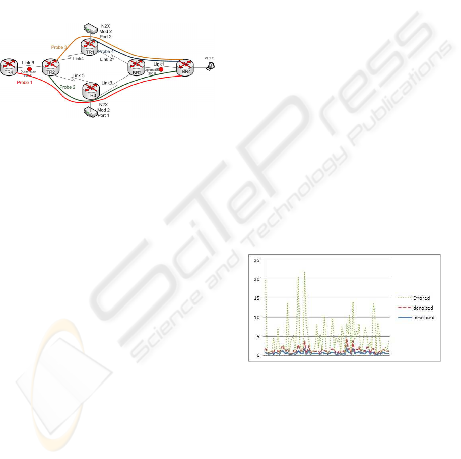
Figure 1 shows a test bed with the four probes

(traveling from right to left) and two of the links

(Link1 and Link6) were stressed with an extended

ping of 200 Bytes. The other source of disturbance

was the trafﬁc from the Agilent router tester (N2X).

The condition of the network remains unchanged dur-

ing the CSLA operation.

Figure 1: Testbed Setup with a mixture of extended pings

and N2X trafﬁc.

6.2 Use of Data from Test Bed

The data obtained from the CSLA is in the form of

accumulative hop-wise round trip time, the following

steps are followed to process the data for obtaining

two matrices; a matrix of end to end delays and a ma-

trix of link level delays.

A parsing software, written in java, extracts link

delays and end to end delays in the form of two ma-

trices. From the accumulative round trip time from

source to each hop, hop to hop delays are calculated to

form the delay matrix. From the accumulative round

trip time (from the source to the destination), end to

end delay matrix is determined. This data has been

used as a baseline for judging the accuracy of the

SCS.

The WGN was simulated through a Matlab based

function and measured link delays were converted

into the noisy link delays. This noisy data was used

as an input to SCS. We expected SCS to denoise this

noisy data in such a way that the denoised link delays

are closer to measured link delays.

As part of the SCS, we needed to apply a BSS

technique as a sparse coding method for determining

the orthogonalmatrix W so that the components s

in s

= Wx have as sparse distributions as possible. We ap-

plied NNMF for this purpose. The end to end link de-

lays obtained from CSLA were input to NNMF. The

Matlab tool NMFpack (Hoyer, 2004) had been used

for NNMF factorization . The NMFpck Matlab pack-

age implements and tests NNMF with the feature of

sparsity. Various combinations of measured link de-

lays and the routing matrix with various sparsity lev-

els were tried to get s

as sparse as possible. These

sparse estimation of s

were input to step 2 of the im-

plementation of SCS as described Section 3.

6.3 Comparison of Measured, Errored,

and Denoised Link Delays

The results have been displayed in six diagrams (Fig-

ure 2 to Figure 7). Each diagram representing one

link, from Link1 to Link6. In each diagram, three

types of data lines are shown:

1. the actual measurement of the link delays col-

lected from CSLA is shown as solid lines in

graphs,

2. the link delays after the introduction of the error

are shown as the dotted lines,

3. the denoised link delays after the application of

SCS are shown as dashed lines.

The vertical axis represents the link delays and hori-

zontal axis is the number of samples at various times.

It is clear from these six graphs that the denoised

link delays are very close to the actual link delays.

The errored link delays were input to SCS and the es-

timated (denoised) values of link delays are close to

the measured values. This shows that the SCS has

successfully denoised the noisy link delay data and

the denoised data is in the proximity of benchmarks.

Figure 2: Comparison of measured, errored, and denoised

link delays on Link1.

7 CONCLUSIONS

High quality trafﬁc measurements are a key to suc-

cessful network management. Direct observation of

the desired statistics in a network is not possible with-

out the special cooperation of the internal network

resources. Network tomography facilitates indirect

estimation of the desired network parameters. Vari-

ous sources introduce errors in the estimated parame-

DENOISING NETWORK TOMOGRAPHY ESTIMATIONS

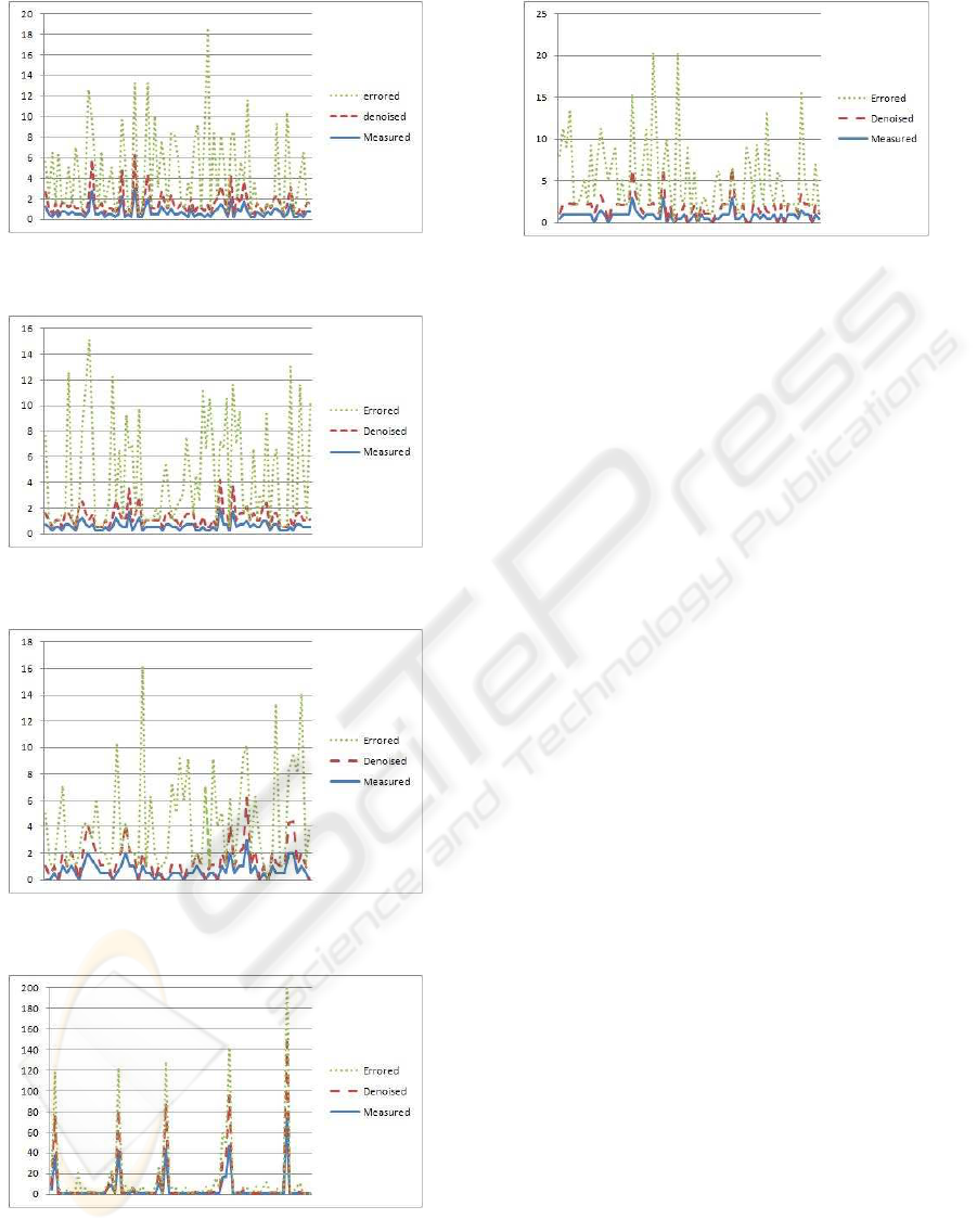
Figure 3: Comparison of measured, errored, and denoised

link delays on Link2.

Figure 4: Comparison of measured, errored, and denoised

link delays on Link3.

Figure 5: Comparison of measured, errored, and denoised

link delays on Link4.

Figure 6: Comparison of measured, errored, and denoised

link delays on Link5.

ters and reduce the effectiveness of the estimated pa-

rameters. We applied the technique of sparse shrink-

age coding (SCS) to denoise the network tomography

Figure 7: Comparison of measured, errored, and denoised

link delays on Link6.

model with errors. To ﬁt well to our research objec-

tives, we modiﬁed SCS by replacing ICA with NNMF

to get all the positive values in the estimated link de-

lay matrices. The results obtained from the laboratory

test bed based simulations proved that SCS success-

fully denoised the link delays. The comparison of de-

noised link delays with the error free benchmark data

showed them very close to each other.

REFERENCES

Castro, R., Coates, M., Liang, G., Nowak, R., and Yu, B.

(2004). Network tomography: Recent developments.

In Statistical Science. Volume 9, 499–517.

Cichocki, A., Zdunek, R., Phan, A. H., , and ichi Amari,

S. (2009). Nonnegative Matrix and Tensor Factor-

izations: Applications to Exploratory Multi-way Data

Analysis and Blind Source Separation. Wiley.

Clemm, A. (2006). Network management fundamentals,

ACM SIGMETRICS Performance Evaluation Review.

Cisco Press.

Coates, M. and Nowak, R. (2001). Network tomography for

internal delay estimation. In 2001 IEEE International

Conference on Acoustics, Speech, and Signal Process-

ing, Proceedings (ICASSP’01). IEEE.

Hoyer, P. (2004). Non-negative matrix factorization with

sparseness constraints. In The Journal of Machine

Learning Research. MIT Press Cambridge, MA, USA,

Volume 5.

Hyvarinen, A. (1999). Sparse code shrinkage: Denoising of

nongaussian data by maximum likelihood estimation.

In Neural Computation. Volume 11, 1739–1768, MIT

Press.

Systems, C. (2010). NetFlow Services Solutions Guide.

available at www.cisco.com.

Vardi, Y. (1996). Network tomography: Estimating source-

destination trafﬁc intensities from link data. In Jour-

nal of the American Statistical Association. Volume

91, 365–377.

Zhao, Q., Ge, Z., Wang, J., and Xu, J. (2006). Robust

trafﬁc matrix estimation with imperfect information:

Making use of multiple data sources. In ACM SIG-

METRICS Performance Evaluation Review. Volume

34, 144.

DCNET 2010 - International Conference on Data Communication Networking