
BEARING-ONLY SAM USING A MINIMAL INVERSE DEPTH
PARAMETRIZATION
Application to Omnidirectional SLAM
Cyril Joly and Patrick Rives
INRIA Sophia Antipolis M´editerran´ee, 2004 route des Lucioles, Sophia Antipolis Cedex, France
Keywords:
Simultaneous localization and mapping (SLAM), Smoothing and mapping (SAM), Extended Kalman filter
(EKF), Bearing-only, Inverse depth representation.
Abstract:
Safe and efficient navigation in large-scale unknown environments remains a key problem which has to be
solved to improve the autonomy of mobile robots. SLAM methods can bring the map of the world and the
trajectory of the robot. Monucular visual SLAM is a difficult problem. Currently, it is solved with an Extended
Kalman Filter (EKF) using the inverse depth parametrization. However, it is now well known that the EKF-
SLAM become inconsistent when dealing with large scale environments. Moreover, the classical inverse depth
parametrization is over-parametrized, which can also be a cause of inconsistency. In this paper, we propose to
adapt the inverse depth representation to the more robust context of smoothing and mapping (SAM). We show
that our algorithm is not over-parameterized and that it gives very accurate results on real data.
1 INTRODUCTION
Simultaneous localization and mapping (SLAM) is a
fundamental and complex problem in mobile robotics
research which has mobilized many researchers since
its initial formulation by Smith and Cheeseman
((Smith and Cheeseman, 1987)). The robot moves
from an unknown location in an unknown environ-
ment and proceeds to incrementally build up a navi-
gation map of the environment, while simultaneously
using this map to update its estimated position. Tra-
ditional methods are based on the extended Kalman
filter (EKF). It is now well known that EKF based
methods yield inconsistencies ((Julier and Uhlmann,
2001; Bailey et al., 2006a)). This is essentially due
to linearization errors. Furthermore, these algorithms
suffer from computational complexity (O(N
2
) where
N is the number of landmarks in the map).
The FastSLAM method, introduced by Thrun and
Montemerlo ((Montemerlo et al., 2003)), is based on
the particle filter. Each position is approximated by a
set of M random particles and one map is associated to
each particle. It can be shown that MlogN complex-
ity is achievable. However, the algorithm is sensitive
to the number of particles chosen. Furthermore, the
issue of particles diversity can make the FastSLAM
inconsistent ((Bailey et al., 2006b)).
In the above-mentionedmethods, SLAM is solved
as a filtering problem: the state-space contains only
the state of the robot at the current time and the state
of the map. SLAM can also be stated as a smooth-
ing problem: the whole trajectory is taken into ac-
count (Thrun and Montemerlo, 2006; Dellaert and
Kaess, 2006). This approach is referred as simulta-
neous smoothing and mapping (SAM). Although it is
based on the linearization of the equations, the ap-
proach gives better results than EKF because all the
linearization points are adjusted during the optimiza-
tion.
A very interesting problem is the monocular vi-
sual SLAM which is also referred as Bearing-Only
SLAM. Since camera does not measure directly the
distance between the robot and the landmark, there
is an observability issue. In standard approach, land-
marks are initialized with a delay. Recent approaches
try to avoid this and propose undelayed formulation.
The method presented in (Civera et al., 2008) consists
in changing the parametrization of the landmarks.
This parametrization includes the location of the first
position where the landmark was observed and the in-
verse depth between the landmark and this position.
Also the latter algorithm produces good results
in real situations, it has some drawbacks. First,
the parametrization of the landmarks is not minimal.
Then, this parametrization is often associated with the
EKF (although it is inconsistent).
281
Joly C. and Rives P. (2010).
BEARING-ONLY SAM USING A MINIMAL INVERSE DEPTH PARAMETRIZATION - Application to Omnidirectional SLAM.
In Proceedings of the 7th International Conference on Informatics in Control, Automation and Robotics, pages 281-288
DOI: 10.5220/0002949702810288
Copyright
c
SciTePress

In this paper, we propose a new way to implement
the inverse depth parametrization by using a SAM ap-
proach. First, the underlying hypothesis of the SLAM
and the general equations are given in section 2. Then,
section 3 presents the SAM algorithm and the par-
ticularities of the inverse depth parametrization with
SAM. Section 4 gives some elements of comparison
between the EKF and the SAM approach. Finally, re-
sults are presented and discussed on real data acquired
by an omnidirectional camera on board of a mobile
robot.
2 BEARING-ONLY SLAM
2.1 Notation and Hypotheses
In the following, we denote:
• x
t
the robot state at time t.
• u
t
the control inputs of the model at time t.
• m
(i)
the i
th
-landmark state. Concatenation of all
landmarks state is m
• z
t(i)
the measurements of landmark i at t. Con-
catenation for all the landmark is z
t
In this paper, we propose to compare two methods
for computing the robot and landmarks states: a new
implementation of the SAM algorithm and the classi-
cal EKF. Both methods use the same hypotheses:
• the robot state x
t
is modeled as a Markov chain,
• conditioned to all the trajectory and the map, mea-
surements at time t depend only on x
t
and m and
are independent of measurements at other time.
Finally, the densities functions for the prediction of
the state of the robot and the observationsare assumed
to be Gaussian:
p(x
t
|x
t−1
,u
t
) = N (f(x
t−1
,u
t
),Q
t
)
p(z
t
|x
t
,m) = N (h(x
t
,m),R
t
)
(1)
where f and h are the prediction and observation func-
tions, Q
t
and R
t
the covariance matrices of the model
and the measurements.
2.2 Camera Motion
Let us consider a standard 6DOFs BO-SLAM config-
uration, i.e. the robot moves in the 3D space and ob-
serves 3D-landmarks with a camera. No more sensor
is considered (no odometry and no IMU). The robot
position at time t is given by its Euclidian coordinates
(r
t
= [x
t
,y
t
,z
t
]
T
) and its orientation by a quaternion
(q
t
).
Since we do not measure the linear and angular ve-
locities, they are estimated in the state. Linear veloc-
ity is defined in the global frame as v
t
= [v
x
t
,v
y
t
,v
z
t
]
T
and angular velocity is defined in the camera frame as
Ω
t
= [ω
x
t
,ω
y
t
,ω
z
t
]
T
.
Furthermore, we assume that constant linear and
angular accelerations act as an input on the system
between t and t + 1. It produces increments V
k
and
Ω
k
. They are modeled as Gaussian white noise with
zero mean. However, the velocity is not exactly con-
stant between two time steps, so that the position and
rotation are not exactly given by the integration of the
velocities defined in the state. We take that into ac-
count by adding two error terms (ν
v
and ν
ω
) in the
model (they are taken as Gaussian white noise).
Finally, the function f which stands for the camera
motion is given by:
x
k+1
=
r
k+1
q
k+1
v
k+1
Ω
k+1
=
r
k
+ (v
k
+ V
k
+ ν
v
)∆t
q
k
× q((Ω
k
+ Ω
k
+ ν
ω
)∆t)
v
k
+ V
k
Ω
k
+ Ω
k
(2)
where q(u) is the quaternion defined by the rotation
vector u.
2.3 Inverse Depth Representation
It is well known that several observations are neces-
sary to estimate a landmark. Indeed, a camera gives
a measurement of the direction of the landmarks, but
not their distance. So, landmarks initialisation is de-
layed when using the classical euclidian representa-
tion (a criterion based on the parallax is generally
used). However, landmarks can bring bearing infor-
mation when the depth is unknown. An interesting
solution was given by Civera et al ((Civera et al.,
2008)). It consists in using a new landmark repre-
sentation based on the inverse depth. In this scheme,
a 3D point (i) can be defined by a 6D vector:
1
y
(i)
=
x
(i)
y
(i)
z
(i)
θ
(i)
φ
(i)
ρ
(i)
T
(3)
where x
(i)
, y
(i)
, z
(i)
are the euclidian coordinates of
the camera position from which the landmark was ob-
served for the first time; θ
(i)
, φ
(i)
the azimuth and ele-
vation (expressed in the world frame) definining unit
directional vector d(θ
(i)
,φ
(i)
) and ρ
(i)
encodes the in-
verse of the distance between the first camera position
and the landmark. So, we can write:
m
Euclidian state
(i)
=
x
(i)
y
(i)
z
(i)
+
1
ρ
(i)
d(θ
(i)
φ
(i)
)
d =
cosφ
(i)
cosθ
(i)
cosφ
(i)
sinθ
(i)
sinφ
(i)
T
(4)
1
in the following, (i) stands for the landmark number.
Parenthesis are used for landmarks in order to avoid confu-
sion between the time index and landmarks index.
ICINCO 2010 - 7th International Conference on Informatics in Control, Automation and Robotics
282

Figure 1: Data association for a loop closure. The angle
between the two views is close to π. This case shows the
advantage of the omnidirectional camera. Such loop clo-
sure would have been impossible with a perspective camera
looking forward.
The main advantage of this representation is that
it satisfies linearity condition for measurement equa-
tion even at very low parallax. According to (Civera
et al., 2008),landmarks can be initialized with only
one measurement.
2.4 Measurement Equation
2.4.1 Specificity of the Omnidirectional Camera
Model
3D points are observed by an omnidirectional camera,
which is the combination of a classical perspective
camera and a mirror. For the low-level image process-
ing, we use algorithms specifically designed to deal
with omnidirectional images (see (Hadj-Abdelkader
et al., 2008) for more details). An example of data as-
sociation in omnidirectional images is given on Fig 1.
First, Harris points are extracted from the current im-
age. Data association with the points extracted from
the previous image is performed thanks to a Sift de-
scriptor. Finally, we obtain a set of matched points of
interest in pixels coordinates.
The points in omnidirectional images are linked to
the landmarks coordinates by the unified projection
model (Barreto, 2003; Mei, 2007). It is done in the
four steps which are recalled below. Let X be the
euclidian coordinates of a point in the camera frame:
1. First, X is projected onto the unit sphere:
X
s
=
X
||X ||
= [X
s
Y
s
Z
s
]
2. The third coordinate of X
s
is shifted by ξ (mirror
parameter):
˜
X
s
= [X
s
Y
s
Z
s
+ ξ]
3. Then, the result is projected onto the unit plane:
u = [
X
s
Z
s
+ξ
Y
s
Z
s
+ξ
1]
4. Finaly, the result is projected onto the image by
p = Ku where K is the calibration matrix of the
system.
In the following, let us write h
1
the function that
returns p from X :
p = h
1
(X ) (5)
2.4.2 Final Measurement Equation
It is shown in (Civera et al., 2008) that the Euclidian
coordinates of landmark (i) in camera frame at time t
are proportional to:
h
2
(y
(i)
,r
t
,q
t
) = R
CW
t
×
×
ρ
(i)
x
(i)
y
(i)
z
(i)
− r
k
+ d(θ
(i)
,φ
(i)
)
where R
CW
t
is the rotation matrix relative to camera
frame and world frame. It is the transpose of the rota-
tion matrix associated to q
t
.
Finally, the measurement equation h is given by:
h = h
1
◦ h
2
(6)
3 SMOOTHING AND MAPPING
3.1 SAM Strategy
In this paper, we propose a SAM method for comput-
ing the states of the robot and the landmarks. So, we
are trying to obtain p(x
0:t
,m|z
0:t
,u
1:t
), which is the
joint probability of the trajectory and the map when
all the measurements and inputs are known. So, the
state contains all the trajectory of the robot and the
landmarks. However, SAM methods can be imple-
mented in real-time due to the block structure of the
information matrix and the use of re-ordering rules
((Dellaert and Kaess, 2006)).
3.2 SAM Equations
With the previous hypotheses, and assuming that no
prior knowledge is available for the landmarks, the
pdf of the trajectory and landmarks can be formulated
as:
p(x
0:t
,m|z
0:t
,u
1:t
) ∝ p(x
0
) p(z
0
|x
0
,m)×
t
∏
k=1
[p(x
k
|x
k−1
,u
k
) p(z
k
|x
k
,m)]
(7)
Taking the logarithm of (7), and assuming that the
functions f and h can be linearized around the ap-
proximated trajectory defined by µ
T
= [µ
x
0:t
T
,µ
m
T
]
T
,
log p(x
0:t
,m|z
0:t
,u
1:t
) yields:
BEARING-ONLY SAM USING A MINIMAL INVERSE DEPTH PARAMETRIZATION - Application to
Omnidirectional SLAM
283

log p(x
0:t
,m|z
0:t
,u
1:t
) = cst−
1
2
x
T
0
I
0
x
0
+ x
T
0
ξ
0
+
∑
t
k=1
−
1
2
"
x
k
x
k−1
#
T
"
I
−G
T
k
#
Q
−1
k
h
I −G
k
i
"
x
k
x
k−1
#
+
"
x
k
x
k−1
#
T
"
I
−G
T
k
#
Q
−1
k
f
k
µ
x
k−1
,u
k
+ G
k
µ
x
k−1
+
∑
t
k=0
−
1
2
"
x
k
m
#
T
"
(H
x
k
)
T
(H
m
k
)
T
#
R
−1
k
h
H
x
k
H
m
k
i
"
x
k
m
#
+
"
x
k
m
#
T
"
(H
x
k
)
T
(H
m
k
)
T
#
R
−1
k
z
k
− h(µ
x
k
,µ
m
)+
h
H
x
k
H
m
k
i
"
µ
x
k
µ
m
#
(8)
where G
k
is the Jacobian of f with respect to
x
k
, H
x
k
(resp. H
m
k
) is the Jacobian of h with re-
spect to x
t
(resp. m) (the Jacobian are computed at
µ). I
0
and ξ
0
are the information matrix and vec-
tor associated to x
0
. If no prior information is avail-
able on x
0
, we set these variables to zero. Equation
(8) shows that log p(x
0:t
,m|z
0:t
,u
1:t
) is quadratic in
x
T
0:t
, m
T
T
. Therefore, p(x
0:t
,m|z
0:t
,u
1:t
) is Gaus-
sian, and the computation of the information parame-
ters are provided by (8). This yields to a sparse matrix
I
2
which simplifies the recovering of the mean and
covariance.
3.3 SAM Implementation
SAM is a filtering algorithm which uses all the data
to compute all the trajectory of the robot and the map.
It needs a prediction of all the trajectory and the po-
sitions of the landmarks. To simulate real time con-
ditions, we decide to use it incrementally (instead of
using once all the measurements). Let us assume that
we have already an estimation of µ
x
1:t−1
and µ
m
. When
the inputs and measurements are available, we update
our estimation in two steps:
1. First, we compute a prediction of µ
x
t
by applying f
2. Then, we compute I and ξ with Eq. (8)
3. µ is given by I
−1
ξ
Usually, the computation of I and ξ is done several
times up to convergence. However, we add only one
pose at each step. Thus, one iteration is enough in
practice with our implementation.
2
Sparseness results from the classical assumption that
measurement of landmark (i) is independent of measure-
ment of landmark ( j) 6= (i) (R
k
matrix is block diagonal).
3.4 Minimal Landmark
Parametrization
3.4.1 Definition of the Parametrization
Let us discuss about the expression of the vector m
that is estimated in the SAM algorithm. We use an
inverse depth representation in order to initialize m at
the first iteration. However, the inverse depth repre-
sentation is not minimal since it uses a 6D vector to
encode a 3D point. We can arbitrarily fix the three
first components and compute the three others. Thus,
the 3 last components are enough to represent a land-
mark in the state if we fix the first ones. Now, let us
assume that 3 first components of y
(i)
are fixed to ˜x
(i)
,
˜y
(i)
and ˜z(i), so that we have m
(i)
= [θ
(i)
φ
(i)
ρ
(i)
]
T
.
However, we can not choose an arbitrary value for
˜x
(i)
, ˜y
(i)
and ˜z(i) if the goal is to insert m
(i)
in the filter
at the first iteration. Indeed, the linearity constraints
has to be respected, which implies that the approx-
imated trajectory has to be close enough to the true
one. To do that, ˜x
(i)
, ˜y
(i)
and ˜z
(i)
are fixed to µ
x
k
(as-
suming that first observation of landmark (i) is at time
k). Choosing any other value would lead to delay the
initialization since we can not guarantee that the an-
gles will be close enough.
Finally, we can notice that the values chosen for
˜x
(i)
, ˜y
(i)
and ˜z(i) are valid for one iteration of the
SAM algoritnm. Indeed, imagine that a part of the
estimated trajectory has changed significantly after
several time steps (because of a loop closure for ex-
ample). The values of the fixed coordinates have to
be update for the next step in the same way than µ
x
.
Reader should note that this is not an “ estimation ”
(in a filter point of view) of ˜x
(i)
, ˜y
(i)
and ˜z
(i)
but a shift
of equilibrium point in order to optimize the validity
of the linearization. We do not compute the jacobian
of h with respect to these fixed components.
3.4.2 Discussion
The parametrization presented in the previous para-
graph takes advantage of the inverse depth represen-
tation but remains minimal since only 3 parameters
are estimated. Using a minimal representation reduce
the risk of “ falling in local minima ”. Furthermore,
we can show that keeping the six variables in the es-
timation would lead to severe inconsistencies in the
case of SAM. Assume for example that landmark (i)
was first observed at time k and that we use the six
variables in m
(i)
. At time k, the three first variables of
m
(i)
are fully correlated with r
k
. Let us examine what
happens for each new observation of m
(i)
for t > k:
ICINCO 2010 - 7th International Conference on Informatics in Control, Automation and Robotics
284
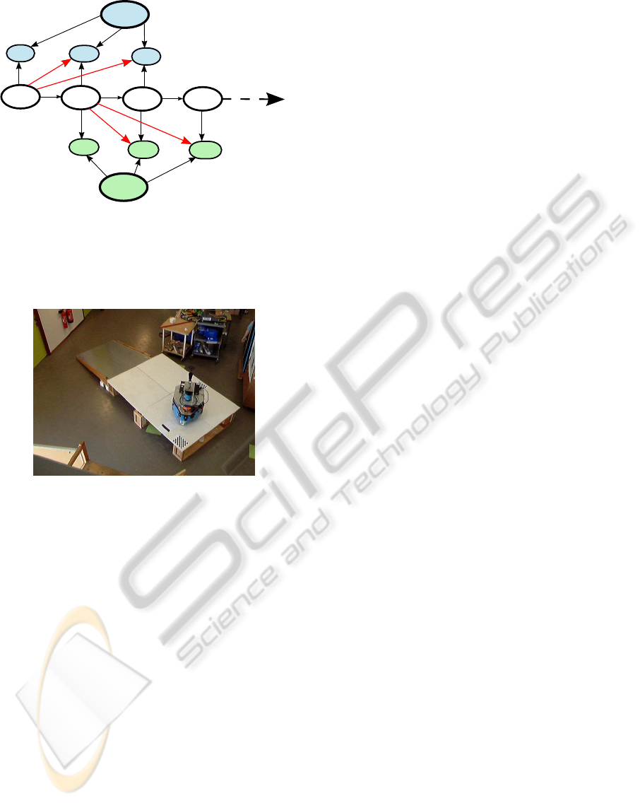
m
(1)
z
0,(1)
z
1,(1)
z
2,(1)
m
(2)
z
1,(2)
z
2,(2)
z
3,(2)
x
0
x
1
x
2
x
3
(a)
Figure 2: Bayesian network in the case of 2 landmarks.
Black links indicates normal links of the network. The red
links indicates spurious links due to over-parametrization
for the EKF case (they are not present with the SAM).
Figure 3: Photo of the experiment.
1. First, the observation will give information about
the current variable x
k
and m
(i)
. This gain of in-
formation implicitly improves the estimation of
all the other variables of the filter by inference,
including r
(k)
2. Then, we should remember that the first 3 com-
ponents of m
(i)
are fully correlated with r
k
which
implies that the information added on x
(i)
, y
(i)
and
z(i) are directly propagated up to r
k
.
The second source of information gathered by r
k
is spurious information. In fact, the full inverse depth
parametrization adds shorcuts in the Bayesian Graph
associated to x and m (Figure 2). With this model,
the measurement of landmark (i) depends directly on
the current robot pose, the landmark and the first po-
sition of observation. The second hypothesis given
in paragraph 2.1 is not satisfied. In practice, such
implementation of the SAM algorithm will lead to di-
vergence.
Finally, an intuitive way to understand the theoret-
ical differences between the EKF formulation and the
minimal SAM representation is to examine the basic
properties of the measurement function:
1. in the case of EKF, h is a function of r
k
, x
t
and
m
(i)
. So, we have z
t
= h(r
k
,x
t
,m
(i)
),
2. in the case of minimal SAM representation, h is a
function of x
t
and m
(i)
parameterized by µ
x
k
. So,
we have z
t
= h
µ
x
k
(x
t
,m
(i)
).
4 COMPARISON WITH THE EKF
In this section, we propose to compare some aspects
of the EKF-SLAM with the SAM. First, it is now well
known that the EKF algorithm is inconsistent. It was
shown in simulations by Tim Bailey (Bailey et al.,
2006a). Moreover, Simon Julier made a proof of the
inconsistency in the case of a static Robot (Julier and
Uhlmann, 2001).
More recently Huang shown the general inconsis-
tency in the case of 3 degrees of freedom SLAM by
an analysis of observability ((Huang et al., 2008)). In-
deed, an observability of the 3DOF-SLAM shows that
the system is unobservable and that the observability
matrix has a nullspace of dimension 3. Intuitively, it
corresponds to a rigid motion of the whole system (2
translations and one rotation). However, the authors
of (Huang et al., 2008) shown that the observability
matrix associated to the system linearized by the EKF
has a nullspace of dimension 2. This corresponds to
spurious information gain in rotation.
They also present an other filter derivated from the
EKF (the The First-Estimates Jacobian EKF SLAM
(FEJ-EKF)) which does not update the linearization
points of the landmarks. This new filter respects the
observabilty nullspace dimension. So, Huang claims
that the root of the EKF inconsistency is the updates
of equilibrium points. We can notice that the for-
mulation of the SAM algorithm guarantees that
the linearization points for the landmarks are the
same for all the observations. In consequence, we
can guess that the good properties of the FEJ-EKF are
kept by the SAM algorithm.
5 RESULTS
5.1 Experimental Testbed
Both algorithms were tested with true data acquired
by a mobile robot in an indoor environment. The tra-
jectory length is about 15m. All the results were ob-
tained in the case of pure bearing-only SLAM (no
odometry).
BEARING-ONLY SAM USING A MINIMAL INVERSE DEPTH PARAMETRIZATION - Application to
Omnidirectional SLAM
285
−2 0 2 4 6 8 10 12
−10
−8
−6
−4
−2
0
2
x coordinate
y coordinate
(a)
0
5
10
−10
−8
−6
−4
−2
0
0
0.2
0.4
0.6
0.8
1
x coordinate
y coordinate
z coordinate
(b)
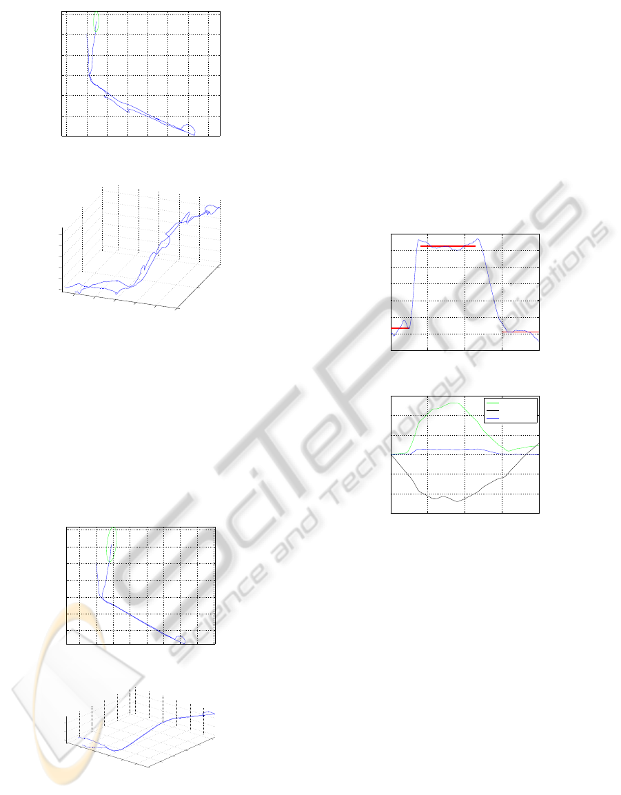
Figure 4: Trajectory provided by the EKF-SLAM.
In order to test the capability of the algorithms to
estimate the 6 DOF of the robot, we made a plateform
at 35cm high from the ground (Figure 3). To access
to this plateform, the robot is driven on a 180cm long
ramp. This gives us a ground truth concerning the
angle of the trajectory of the robot during its “ climb ”:
γ = arcsin(35/180) ≈ 11.2deg (9)
−1 0 1 2 3 4 5 6 7
−4
−3
−2
−1
0
1
2
(a)
0
1
2
3
4
5
−4
−3
−2
−1
0
1
0
0.2
0.4
x coordinate
y coordinate
z coordinate
(b)
Figure 5: Trajectory provided by the SAM algorithm.
Furthermore, the robot is submitted to high
changes in rotation velocity. Particulary, the robot
makes a turn just before climbing on the plateform.
Then, the robot rotates on itself (without translation)
once it is on the plateform. Some pictures of the ex-
periment are proposed on Figure 3. As the camera
is not mounted on the center of rotation of the robot,
we expect to see a semicircle in the trajectory. The
end of the trajectory consists in going down to the
ground and moving in the plane. We also used the
fact that the robot came back close to the first position
to force a loop closure (the loop closure correspond to
the data association shown on Fig 1). Both algorithms
are tested with exactly the same data (the image pro-
cessing is done off-line). Finally, even if we do not
0 100 200 300 400
−0.1
0
0.1
0.2
0.3
0.4
0.5
0.6
Sample number
z coordinate
(a)
0 100 200 300 400
−6
−4
−2
0
2
4
6
Sample number
x,y,z coordinates
x coordinate
y coordinate
z coordinate
(b)
Figure 6: SAM solution — (a) z coordinate – (b) x, y and
z coordinates: we see the relevance of z with respect to the
main scale (x and y).
have a ground truth on all the trajectory, we have 4
parameters which can be tested:
1. The robot is on the ground during the first part of
the trajectory. So, we expect the z coordinate of
the trajectory to be zero,
2. The angle of the ramp is known. We can use it as
a ground truth,
3. After the climb, the robot movement is parallel to
the ground. So, we expect the z coordinate to be a
constant,
4. The robot is on the ground during the last part of
the trajectory.
ICINCO 2010 - 7th International Conference on Informatics in Control, Automation and Robotics
286

−5 0 5 10 15 20
−20
−15
−10
−5
0
x coordinate
y coordinate
(a)
0
5
10
15
−15
−10
−5
0
5
10
−3
−2
−1
0
1
x coordinate (m)
y coordinate (m)
z coordinate (m)
(b)
Figure 7: Map provided by the SAM algorithm. The trajectory is also plotted in red.
5.2 Results on the EKF
The trajectory given by the EKF is given on Figure 4.
The trajectory starts from the origin. The green ellip-
sis on Figure 4a shows the uncertaintyof the last robot
pose. We can see that there are many discontinuities
in the trajectory at the end due to the loop closure.
This is due to the fact that when the robot observe an
old landmark, the drift accumulated force the filter to
make a discontinuity in the solution. Finally, even if
the trajectory looks fine (we see the different heights
and the semicircle), results of the EKF are not much
impresive.
5.3 Results on the SAM
The results provided by the SAM algorithm are given
on Figure 5 to 7. They look like much interesting than
the EKF-SLAM results. Indeed, the estimation of the
trajectory is very smooth comparing to the one pro-
vided by the EKF. Moreover, we can see that the un-
certainty ellipsis is bigger in the case of the SAM al-
gorithm. This is certainly a manifestation of the EKF
inconsistency: the EKF is over-confident.
Moreover, we were able to compute an approx-
imation of the angle γ with the trajectory by using
the coordinates at the beginning and at the end of the
climb. We got 10.1deg (the ground truth is 11.2deg).
We have just an error of 1.1deg. This confirms the
excellent results provided by the SAM algorithm.
We also checked the relevance of the z coordi-
nate (Figure 6). It appears that the mean value during
the first part of the trajectory is 0.03m with a stan-
dard deviation of 0.03m (first red bar on Figure 6a).
During the second part of the trajectory (after the
climb), the mean value of z is 0.52m (standard devia-
tion: 0.015m). Finally, the mean value of z during the
last part of the trajectory is 0.01 (standard deviation:
0.02m). These results are good: we get the two parts
were z is close from 0 and see a near constant z
during the second part of the trajectory. Then, z values
are scaled with the values of x and y on Figure 6b:
we can see that displacements in z are much smaller
than displacement in x, y. However, the shape of the
z is well estimated, which shows the good precision
of the algorithm. We got similar results with the EKF
algorithm (but with a higher level of noise).
Finally, the map provided by the SAM algorithm
is given on Figure 7. It is quite difficult to interpret
since we do not have any ground truth (the map is
made by interest points selected during the video se-
quence). Nevertheless, we can see on the left part a
wall (close to the zero vertical axis) which seems to
be coherent.
6 CONCLUSIONS
In this paper, we proposed an accurate method to
solve the monocular SLAM problem. To do it,
we used the inverse depth representation for land-
marks and the SAM algorithm for the filtering part.
However, we do not use the whole inverse depth
parametrization as proposed by the original authors.
Indeed, we decide to fix the three first components
of the representation by using the linearization points
provided by the SAM algorithm. Thus, we solved the
over-parametrizationproblemintroduced by the EKF-
version of the algorithm. In consequence, two origins
of inconsitencies are avoided: the one due to the in-
herent inconsistency of EKF, and the one due to the
over-parametrization. This makes our algorithm more
robust than the EKF proposed by Civera et al.
We shown that we had a very good estimation
without any odometry. First, we recovered the angle
of the ramp if good precision. Then the z coordinate
estimation was quite relevant in spite of the small ver-
tical displacements comparing to the x and y coordi-
nates.
Our future work will focus on optimizing the al-
BEARING-ONLY SAM USING A MINIMAL INVERSE DEPTH PARAMETRIZATION - Application to
Omnidirectional SLAM
287

gorithm and implementing a strategy to switch from
inverse depth coordinates to classical euclidian coor-
dinates. Indeed, inverse depth parametrization is very
relevant when parallax is small. Then, classical co-
ordinates can be used. The authors of (Civera et al.,
2007) propose a test to switch from inverse depth co-
ordinates to global ones. We will focus on adapting
this strategy to our algorithm.
REFERENCES
Bailey, T., Nieto, J., Guivant, J., Stevens, M., and Nebot,
E. (2006a). Consistency of the ekf-slam algorithm.
In IEEE/RSJ International Conference on Intelligent
Robots and Systems.
Bailey, T., Nieto, J., and Nebot, E. (2006b). Consistency of
the fastslam algorithm. In IEEE International Confer-
ence on Robotics and Automation.
Barreto, J. P. (2003). General Central Projection Systems,
modeling, calibration and visual servoing. PhD thesis,
Department of electrical and computer engineering.
Civera, J., Davion, A. J., and Montiel, J. M. (2008). Inverse
Depth Parametrization for Monocular SLAM. IEEE
Transactions On Robotics, 24(5).
Civera, J., Davison, A. J., and Montiel, J. (2007). Inverse
depth to depth conversion for monocular slam. In In-
ternational Conference on Robotics and Automation
(ICRA).
Dellaert, F. and Kaess, M. (2006). Square Root SAM: Si-
multaneous Location and Mapping via Square Root
Information Smoothing. Journal of Robotics Re-
search.
Hadj-Abdelkader, H., Malis, E., and Rives, P. (2008).
Spherical Image Processing for Accurate Odometry
with Omnidirectional Cameras. In The Eighth Work-
shop on Omnidirectional Vision.
Huang, G., Mourikis, A., , and Roumeliotis, S. (2008).
Analysis and improvement of the consistency of ex-
tended kalman filter based slam. In Proceedings of
the 2008 IEEE International Conference on Robotics
and Automation (ICRA).
Julier, S. J. and Uhlmann, J. K. (2001). A counter exam-
ple to the theory of simultaneous localization and map
building. In International Conference on Robotics and
Automation (ICRA).
Mei, C. (2007). Laser-Augmented Omnidirectional Vision
for 3D Localisation and Mapping. PhD thesis, Ecole
des Mines de Paris, INRIA Sophia Antipolis.
Montemerlo, M., Thrun, S., Koller, D., and Wegbreit,
B. (2003). FastSLAM 2.0: An Improved Parti-
cle Filtering Algorithm for Simultaneous Localiza-
tion and Mapping that Provably Converges. In In-
ternational Joint Conference on Artificial Intelligence,
pages 1151–1156.
Smith, R. and Cheeseman, P. (1987). On the representation
and estimation of spatial uncertainty. International
Journal of Robotics Research, 5(4):56–68.
Thrun, S. and Montemerlo, M. (2006). The GraphSLAM
Algorithm with Applications to Large-Scale Mapping
of Urban Structures. The International Journal of
Robotics Research, 25(5-6):403–429.
ICINCO 2010 - 7th International Conference on Informatics in Control, Automation and Robotics
288
