
ROAD CRACK EXTRACTION WITH ADAPTED FILTERING AND
MARKOV MODEL-BASED SEGMENTATION
Introduction and Validation
S. Chambon, C. Gourraud, J.-M. Moliard and P. Nicolle
Laboratoire Central des Ponts et Chausses, LCPC, Nantes, France
Keywords:
Fine structure extraction, Evaluation and comparison protocol, Matched filter, Markov model, Segmentation.
Abstract:
The automatic detection of road cracks is important in a lot of countries to quantify the quality of road surfaces
and to determine the national roads that have to be improved. Many methods have been proposed to automat-
ically detect the defects of road surface and, in particular, cracks: with tools of mathematical morphology,
neuron networks or multiscale filter. These last methods are the most appropriate ones and our work con-
cerns the validation of a wavelet decomposition which is used as the initialisation of a segmentation based on
Markovian modelling. Nowadays, there is no tool to compare and to evaluate precisely the peformances and
the advantages of all the existing methods and to qualify the efficiency of a method compared to the state of the
art. In consequence, the aim of this work is to validate our method and to describe how to set the parameters.
1 INTRODUCTION
In many countries, the quality of roads is evalu-
ated by taking into account numerous characteristics:
adherence, texture and defects. Since 1980, many
efforts have been spent for making this task more
comfortable, less dangerous for employees and also,
more efficient and less expensive by using an acquisi-
tion system of road images and by introducing semi-
automatic defect detection, in particular crack detec-
tion. Nowadays, a lot of acquisition systems are pro-
posed, see (Schmidt, 2003), but, as far as we are con-
cerned, even if a lot of automatic crack detections had
been proposed, no method had been widely applied.
In fact, this problem is difficult because road cracks
represent a small part of the images (less than 1.5%
of the image) and is very low contrasted (the signal
of the crack is mixed with the road texture). Actu-
ally, there is no evaluation protocol to compare and to
highlight methods that are well dedicated to this task
and we propose to introduce such a protocol. More-
over, our second aim is to introduce and to validate
our contributions about a multi-scale approach based
on two steps: a binarization with adapted filtering and
a refinement of the binarization by a Markov model-
based segmentation.
First, existing methods are resumed before describing
our approach. Then, we introduce the evaluation pro-
tocol that enables us to validate the new approach and
we give the details of the parameter settings.
2 DETECTION OF ROAD
CRACKS
For this task, three steps can be distinguished: image
acquisition, data storage and image processing. In this
paper, even if the choices for the two first steps are
important, we focus on the image processing step.
Four different kinds of methods exist, see Table 1.
The thresholding methods are the oldest ones and also
the most popular. They are based on histogram analy-
sis (Acosta et al., 1992), on adaptive thresholding (El-
behiery et al., 2005), or on Gaussian modelling (Kout-
sopoulos and Downey, 1993). These techniques are
simple but not very efficient: the results show a lot of
false detections. Some methods are based on morpho-
logical tools (Elbehiery et al., 2005; Iyer and Sinha,
2005; Tanaka and Uematsu, 1998). The results con-
tain less false detections but they are highly depen-
dent on the choice of the parameters. Neuron net-
works-based methods have been proposed to alleviate
the problems of the two first categories (Kaseko and
Ritchie, 1993). However, they need a learning phase
which is not well appropriate to the task. Filtering
81
Chambon S., Gourraud C., Moliard J. and Nicolle P. (2010).
ROAD CRACK EXTRACTION WITH ADAPTED FILTERING AND MARKOV MODEL-BASED SEGMENTATION - Introduction and Validation.
In Proceedings of the International Conference on Computer Vision Theory and Applications, pages 81-90
DOI: 10.5220/0002848800810090
Copyright
c
SciTePress

methods are the most recent. At the beginning, a con-
tour detection has been used but the major drawbacks
lie on using a constant scale, supposing that the width
of the crack is constant and that we suppose that the
background is not as noisy (or textured) as a road sur-
face. This is not realistic and this is why, most of the
filtering methods are based on a wavelet decomposi-
tion (Delagnes and Barba, 1995; Subirats et al., 2006;
Wang et al., 2007; Zhou et al., 2005) or on partial dif-
ferential equations (Augereau et al., 2001). We can
also notice an auto-correlation method (Lee and Os-
hima, 1994) (the authors estimate a similarity coeffi-
cient between patterns that represent simulated cracks
and patterns inside the images). Some methods also
use texture decomposition (Petrou et al., 1996; Song
et al., 1992) (the goal is to find a noise, i.e. the crack,
inside a known texture).
Table 1: State of the art about road crack detection – In
brackets, we give the years of publication.
THRESHOLD
(1992–1999)
(Acosta et al., 1992; Cheng
et al., 1999; Koutsopoulos and
Downey, 1993)
MORPHOLOGY
(1998)
(Tanaka and Uematsu, 1998)
NEURAL
NETWORK
(1991–2006)
(Bray et al., 2006; Chou et al.,
1995; Kaseko and Ritchie,
1993; Ritchie et al., 1991)
MULTI-
SCALE
(1990–2009)
(Chambon et al., 2009;
Delagnes and Barba, 1995;
Fukuhara et al., 1990; Subirats
et al., 2006; Zhou et al., 2005)
3 AFMM METHOD
First, we present the general algorithm of the method:
Adapted Filtering and Markov Model-based segmen-
tation (AFMM) and, second, our contributions in each
of the parts of this algorithm.
3.1 Algorithm
The goal of this algorithm, presented in Figure 1, is
to obtain, steps 1 to 3, a binarization (black pixels
for background and white pixels for the crack) and
a refinement of this detection by using a Markovian
segmentation, step 4,. In the first part, a photometric
hypothesis is used: a crack is darker than the back-
ground (the rest of the road pavement) whereas, in
the second part, a geometric hypothesis is exploited:
a crack is composed of a set of connected segments
with different orientations. The number of scales for
the adapted filtering has to be chosen and depends on
the resolution of the image. By supposing a resolution
of 1 mm per pixel, by choosing 5 scales, a crack with a
width from 2 mm to 1 cm can be detected. Moreover,
the number of directions (for the filtering) also has
to be chosen and, it seems natural to take these four
directions: [0,
π
4
,
π
2
,
3π
4
] that correspond to the four
usual directions used for crack classification. Adapted
filtering is applied in each scale, each directions and
then all the results are merged (mean of the coeffi-
cients). The results of this filtering is used to initialize
the Markov model.
Input
Road images
Initialization
Number of scales and angles
Steps
1. For each scale do Estimate adapted
filter (AF)
2. For each direction do Apply AF
3. Merge AF in all the directions
4. For each scale do
(a) Initialize the sites (Markov)
(b) While not (stop condition) do
Update the sites
Figure 1: Algorithm with adapted filter and Markovian
modelling (AFMM) – Steps 1 to 3 lead to a binary image
using adapted filtering, while step 4 refines this result with
a Markovian modelling.
3.2 Adapted Filtering
The ψ ∈ L
2
(IR
2
) function is a wavelet if:
Z
IR
2
|Ψ(x)|
2
kxk
2
dx < ∞,avec x = (i, j), (1)
where Ψ is the Fourier transform of ψ. The equa-
tion (1) induces that
Z
IR
2
ψ(x)dx = 0. The wavelet
family is defined for each scale s and for each posi-
tion u, by :
ψ
x, ˆu,θ
(x) =
1
2
ψ(R
θ
((x−u)/s)), (2)
where ψ ∈ IR
2
and R
θ
is a rotation of angle θ. One
of the main difficulties to apply a wavelet decompo-
sition is the choice of the mother wavelet ψ. Nu-
merous functions are used in the literature: Haar
wavelet, Gaussian derivatives, Mexican hat filter,
Morlet wavelet. It is very hard to determine which
VISAPP 2010 - International Conference on Computer Vision Theory and Applications
82
one is the best for a given application. In the case of
crack detection, two elements are present: the crack
(if there is a crack) and the background (the road
surface can be viewed as a repetitive texture). The
goal of the crack detection is to recognize a signal,
i.e. the shape is known up to a factor, mixed with
a noise whose its characteristics are known. Con-
sequently, adapted filtering is well designed for the
problem: extracting singularities in coefficients esti-
mated by a wavelet transform. If s is a discrete and
deterministic signal with values stored in the vector
s =
s
1
... s
N
, N the number of samples, and
z =
z
1
... z
N
, is a noisy observation of s, supposed
to be an additive noise: z = s+b. The main hypothe-
sis is that this second-order noise is centered and sta-
tionary, with auto-correlation function φ
bb
of terms
φ
bb
(i, j)
= φ
bb
|i−j|
, independent from the signal s. The
adapted filter h of s is defined by:
h = φ
−1
bb
s. (3)
The crack signal depends on the definition of the
crack. In this paper, like most of the papers of this
domain, crack pixels correspond to black pixels sur-
rounded by background pixels (road pixels). This is
why, in (Subirats et al., 2006), a crack is a piecewise
constant function:
f(x) =
(
−a If x ∈ [−
T
2
,
T
2
]
0 Elsewhere,
(4)
where the factor a and the threshold T have to be de-
termined. It does not correspond to a realistic rep-
resentation of the crack. Because of sub-sampling,
lights, orientation of the camera, the signal is more
like a Gaussian function with zero mean:
f(x) = −a e
−
1
2
(
x
σ
)
2
, (5)
where a is the size of the crack and depends on σ,
the deviation of the Gaussian law, i.e. a =
1
σ
√
(2π)
.
Consequently, the term σ allows to fix the width of
the crack (like threshold T in equation (4)).
3.3 Contribution to Segmentation
The goal of this part is to extract shapes, i.e. cracks,
using the detection maps estimated at the first stage
of the algorithm. The MRF (Markov Random Field)
principle is introduced before the presentation of the
improvements about the initialization of sites and the
updating of the Markov Random Field.
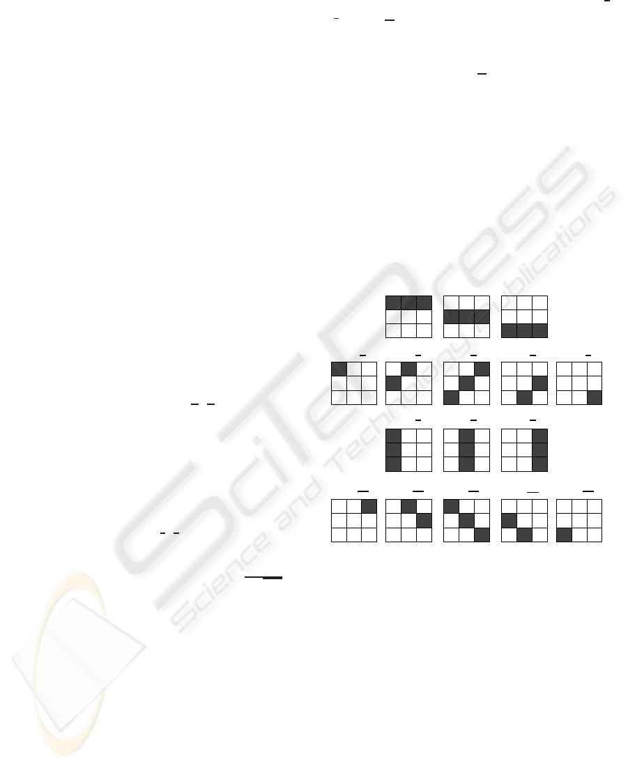
For the first step of segmentation (initialization),
in (Subirats et al., 2006), the sites are of size 3 ×3,
consequently, a regular grid is considered in the im-
age. The four configurationsthat are possible, are rep-
resented in Figure 2. The initialization of the sites is
based on the configuration that maximizes the wavelet
coefficients. More formally, if we denoted γ
2,0
, γ
2,
π
4
,
γ
2,
π
2
and γ
2,
3π
4
, see in the bold rectangle in Figure 2,
the four configurations, the best configuration γ
best
is:
γ
best
= argmax
α∈
[
0..
3π
4
]
m
2,α
, (6)
where m
2,α
is the mean of wavelet coefficients on the
considered configuration γ
2,α
. These four configura-
tions do not represent all the possible and are not re-
alistic configurations. In fact, all these four config-
urations are centered, whereas, it is possible to have
some non-centered configurations. Consequently, we
use a set of configurations that includes this aspect
and we employ a set of sixteen configurations illus-
trated in Figure 2. By modifying the number of con-
figurations, we need to adapt the initialization of sites,
i.e. equation (6).
γ
3,
3ψ
4
γ
0,
3π
4
γ
1,
3π
4
γ
2,
3π
4
γ
4,
3π
4
γ
1,0
γ
3,0
γ
2,0
γ
0,
π
4
γ
2,
π
2
γ
3,
π
2
γ
1,
π
2
γ
3,
π
4
γ
1,
π
4
γ
2,
π
4
γ
4,
π
4
Figure 2: The sixteen configurations of the Markov model
(initialization) – The sites are represented with dark gray
levels.
The image is considered as a finite set of sites denoted
S = {s
1
,... , s
N
}. For each site, the neighborhood is
defined by: V
s
=
n
s
′
|s /∈ V
s
′
& s
′
∈ V
s
⇒ s ∈V
s
′
o
.
A clique c is defined as a subset of sites in S where
every pair of distinct sites are neighbors.
The random fields considered are:
1. The observation field Y = {y
s
} with s ∈ S . Here,
y
s
is the mean of wavelet coefficients on the site.
2. The descriptor field L = {l
s
} with s ∈ S . For this
work, if there is a crack l
s
= 1 elsewhere l
s
= 0.
MRF model is well suited to take into account spatial
dependencies between the variables. Each iteration,
a global cost, or a sum of potentials, that depends on
ROAD CRACK EXTRACTIONWITH ADAPTED FILTERING AND MARKOV MODEL-BASED SEGMENTATION -
Introduction and Validation
83

the values of the sites and the links between neigh-
borhoods, is updated. This global cost takes into ac-
count the site coefficients(computed from the wavelet
coefficients estimated during the first part of the al-
gorithm: adaptive filtering) and the relation between
each site and the sites in its neighborhood (in this pa-
per, it corresponds to the eight neighbors). More for-
mally, the global cost is the sum of all the potentials
of the sites and contains two terms:
u
s
(s) = α
1
u
1
(s) + α
2
∑
s
′
∈V
s
u
2
(s,s
′
), (7)
where V
s
is the neighborhood of site s. The choice
of the values α
1
and α
2
depends on the importance of
each part of the equation (7).
The function u
1
is given by:
u
1
(y
s
,l
s
= 1) =
(
e
ξ
1
(k−y
s
)
2
If y
s
≥ k
1 Elsewhere
and
u
1
(y
s
,l
s
= 0) =
(
e
ξ
2
(y
s
−k)
2
If y
s
< k
1 Elsewhere,
(8)
The parameters ξ
1
, ξ
2
and k have to be fixed
1
. For
the definition of u
2
, we have to determine the num-
ber of cliques. In (Subirats et al., 2006), four cliques
are possible. As there is four configurations in the
previous approach, there is sixteen possibilities. A
8-neighborhood is considering but the potential func-
tion proposed in the precedent work only considers
the difference of orientations between two neighbor-
hoods and not the position between the two sites of
the clique, see Table 2.
Table 2: Function u
2
– This table represents the values of
the function u
2
(s
′
,s) for the four initial configurations of
the sites. In the experiments we have taken the values of the
parameters proposed by the authors (Subirats et al., 2006)
and that give the best results: β
1
= −2, β
2
= −1 and β
3
= 2.
γ
2,0
γ
2,
π
4
γ
2,
π
2
γ
2,
3π
4
γ
2,0
β
1
β
2
β
3
β
2
γ
2,
π
4
β
2
β
1
β
2
β
3
γ
2,
π
2
β
3
β
2
β
1
β
2
γ
2,
3π
4
β
2
β
3
β
2
β
1
Some cases are not penalized with the old config-
uration. For example, these two unfavorable cases are
1
The choice of k is related to the maximal number of
pixels that belong to a crack (it depends on the resolution of
images and hypothesis about the size and configuration of
cracks). We have chosen k in order to consider at most 5%
of the image as a crack. Moreover, our experimentations
have brought us to take ξ
1
=ξ
2
=100.
not penalized: two sites with the same orientation but
with no connection between them, two sites with the
same orientation but their position makes them par-
allel. This is why, with the sixteen possible config-
urations presented in Figure 2, the new variant takes
into account differences of orientations between two
sites (there are 16×16 possibilities) and position of
the two sites (there is eight possibilities because of 8-
connexion). Consequently, the new potential function
u
2
follows these two important rules:
(R
1
) The lower the difference of orientations between
two sites, the lower the potential.
(R
2
) The lower the distance between two sites, the
lower the potential (in this case, distance means
the minimal distance between the extremities of
the two segments).
More formally, if d denotes the Euclidean distance
between the two closest extremities of the sites, with
d ∈ [0, d
max
] (d
max
= 5
√
2), θ
1
and θ
2
, the ori-
entations of respectively s = {s
i
}
i=1..N
s
, and s
′
=
{s
′
j
}
j=1..N
s
′
and θ
e
the angle between the two sites,
the u
2
function is defined by:
u
2
(s
′
,s) = α
2
|2θ
e
−θ
1
−θ
2
|
2π
+
(1−α
2
)
J(NbC) min
i, j
(d(s
i
,s
′
j
))
d
max
−
NbC
3
.
(9)
where NbC indicates the number of elements of the
two sites s and s
′
and J(x) equals 1 if NbC = 0 and 0
elsewhere. The first term is induced by the rule about
the orientations, rule (R
1
), it is zero when the sites
have the same orientation and this orientation is the
same as the orientation between the sites, i.e. θ
e
=
θ
2
= θ
1
. It gives bad costs to configurations where
the sites do not have the same orientation but also the
particular case where they are parallel, see example
(a) in Figure 3. The second and third terms express
the rule (R
2
) about the distances. Two aspects have
to be distinguished: the number of connected pixels,
when the sites are connected, and, on the contrary,
the distance between the sites. It allows to give low
influence to disconnected sites and also to increase
the cost of sites that are parallel but connected, see
example (b) in Figure 3. To study the influence of all
these terms, the equation has been normalized and the
different terms have been weighted.
4 EVALUATION PROTOCOL
For the evaluation of automatic crack detection, there
is no evaluation and comparison protocol proposed in
VISAPP 2010 - International Conference on Computer Vision Theory and Applications
84
(a) (b)
s
0
s
1
s
2
s
3
s
2
s
1
s
3
s
0
θ
0
= θ
1
= θ
2
=
π
4
, θ
3
=
π
2
θ
e1
= 0, θ
e2
=
π
4
and
θ
e3
=
π
2
For s
1
: u
2
=
π
2
−0+ 2
For s
2
: u
2
= 0−1+ 0
For s
3
: u
2
=
π
4
−1+ 0
θ
0
= θ
1
= θ
2
= θ
3
=
π
2
θ
e1
= 0, θ
e2
= θ
e3
=
π
2
For s
1
: u
2
= π−3+ 0
For s
2
: u
2
= 0−1+ 0
For s
3
: u
2
= 0−0+ 2
Figure 3: Illustration of function u
2
– These two examples
of sites with their respective neighborhoods show the be-
havior of potential u
2
with the two considered aspects: ori-
entation and distance. In example (a), with the help of the
orientation term, the configuration s
1
is penalized and s
3
is
less penalized than s
1
. In example (b), with the help of the
two terms on distance, the site s
3
is penalized, compared to
s
2
. On the contrary, the particular case of s
1
is favorable and
it equilibrates the penalty given by the orientations.
the community. However, in all the countries, for es-
timating the quality of the road surface, it is impor-
tant to know exactly the size and the width of the de-
fects, i.e. to detect precisely the defect. This is why,
it seems important to characterize quantitatively the
performance of the methods. For building this kind
of protocol, it is necessary, first, to choose the tested
images, second, to choose how to build reference seg-
mentations, and, third, to determine the criteria used
for the quantitative analysis.
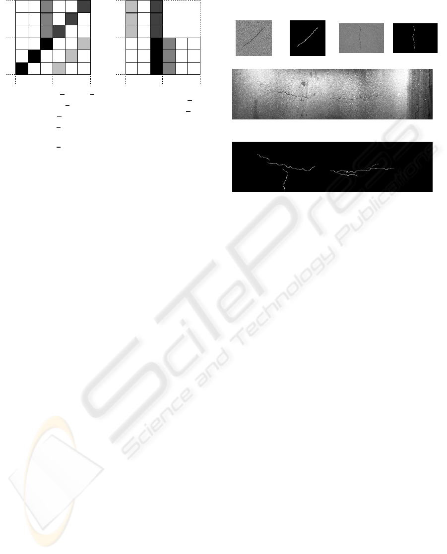
4.1 Tested Images
The most difficult is to propose images with a ref-
erence segmentation or a ”ground truth” segmenta-
tion. On the first hand, we create synthetic images
with a simulated crack. As shown in figure 4, the re-
sult is not enough realistic and, on the second hand,
we have taken a real image with no defect and we
have added a simulated defect. The result is more re-
alistic but the shape of the crack (which is randomly
chosen) does not seem enough realistic. This is why,
it appears important to propose a set of real images
with manual segmentations that are enough reliable to
be considered as reference segmentations or ”ground
truth” segmentations. To resume, the two first kinds
of images allow to propose an exact evaluation and
to well illustrate the behavior of the method in theo-
retical cases whereas the last kind of images allows
to validate the work on real images with a ”pseudo”
ground truth.
Synthetic
image
Ground truth
Real image +
simulated
defect
Ground truth
Real image manually segmented
Reference segmentation or pseudo ground truth
segmentation
Figure 4: Tested images.
4.2 Reference Segmentation
For real images, we briefly explain how the manual
segmentation is validated. Four experts manually give
a segmentation of the images with the same tools and
in the same conditions. Then, the four segmentations
are merged, following these rules:
1. A pixel marked as a crack by more than two ex-
perts is considered as a crack pixel;
2. Every pixel marked as a crack and next to a pixel
kept by step 1 or 2 is also considered as a crack.
The second rule is iterative and stops when no pixel
is added. Then, the result is dilated with a structuring
element of size 3×3.
In this part, we distinguish two datasets of real im-
ages. First, we have work with 10 images, in order to
validate our manual segmentation and to determine
how to fix the parameters of the proposed method.
This first dataset is called initial dataset. The sec-
ond one contains 32 images to complete the evalua-
tion and we called it the complementary dataset.
Initial Dataset. To evaluate the reliability of the ref-
erence segmentations, we estimate, first, the percent-
age of covering between each operator, and, second,
the mean distance between each pixel (detected by
only one expert and not kept in the reference image)
and the reference segmentation. Table 3 compares the
results for these 10 first images. We can notice that the
first 4 images are the most reliable because the mean
error is less than 2 pixels. On the contrary, the last
6 images are less reliable but they are also the most
difficult to extract a segmentation.
ROAD CRACK EXTRACTIONWITH ADAPTED FILTERING AND MARKOV MODEL-BASED SEGMENTATION -
Introduction and Validation
85
Complementary Dataset. The same technique is
used for establishing the reference segmentations
with 32 images. By analyzing the results for criteria
D., presented in Table 3, we decided to classify the 42
tested images in 3 categories:
1. Reliable: All the images have obtained D < 2 and
it means that all the operators have selected areas
that are quite close to each other and the segmen-
tation is reliable.
2. Quite reliable: All the images have obtained
2 ≤ D < 8, it means that some parts of the crack
are not easy to segment and there are locally big
errors.
3. Ambiguous: All the images have obtained D ≥8.
It clearly show that the images are really difficult
to segment and in most of the cases, it means that
some parts are detected as a crack whereas they
are not a crack and reversely.
Table 3: Manual segmentation comparison for establishing
the reference segmentations – For each image, we give the
percentage of pixels that are preserved in the final reference
segmentation compared to the size of the image (F), the per-
centage of covering between 2, 3 and 4 segmentations (over
all the pixels marked as crack by the 4 experts) and the sum
of them (S). For all the crack pixels not preserved in the
final reference segmentation, the mean distance to this seg-
mentation is given, noted D.
Images F (%) 2 (%) 3 (%) 4 (%) S (%) D (pix)
37 0.45 28.87 9.79 1.59 40.25 1.48
42 0.4 26.69 14.59 4.2 45.48 1.45
46 0.72 27.53 11.66 2.33 41.52 1.41
40 0.44 34.3 19.01 5.87 59.18 1.03
463 0.17 23.46 5.95 0.39 29.8 1.4
936 0.41 23.52 7.41 0.9 31.83 7.05
41 0.33 22.64 7.31 1.33 31.28 3.56
23 0.6 24.12 9.41 2.45 36.58 2.23
352 1.01 25.69 11.52 2.15 39.36 4.75
88 1.44 22.74 8.23 1.23 32.2 2.76
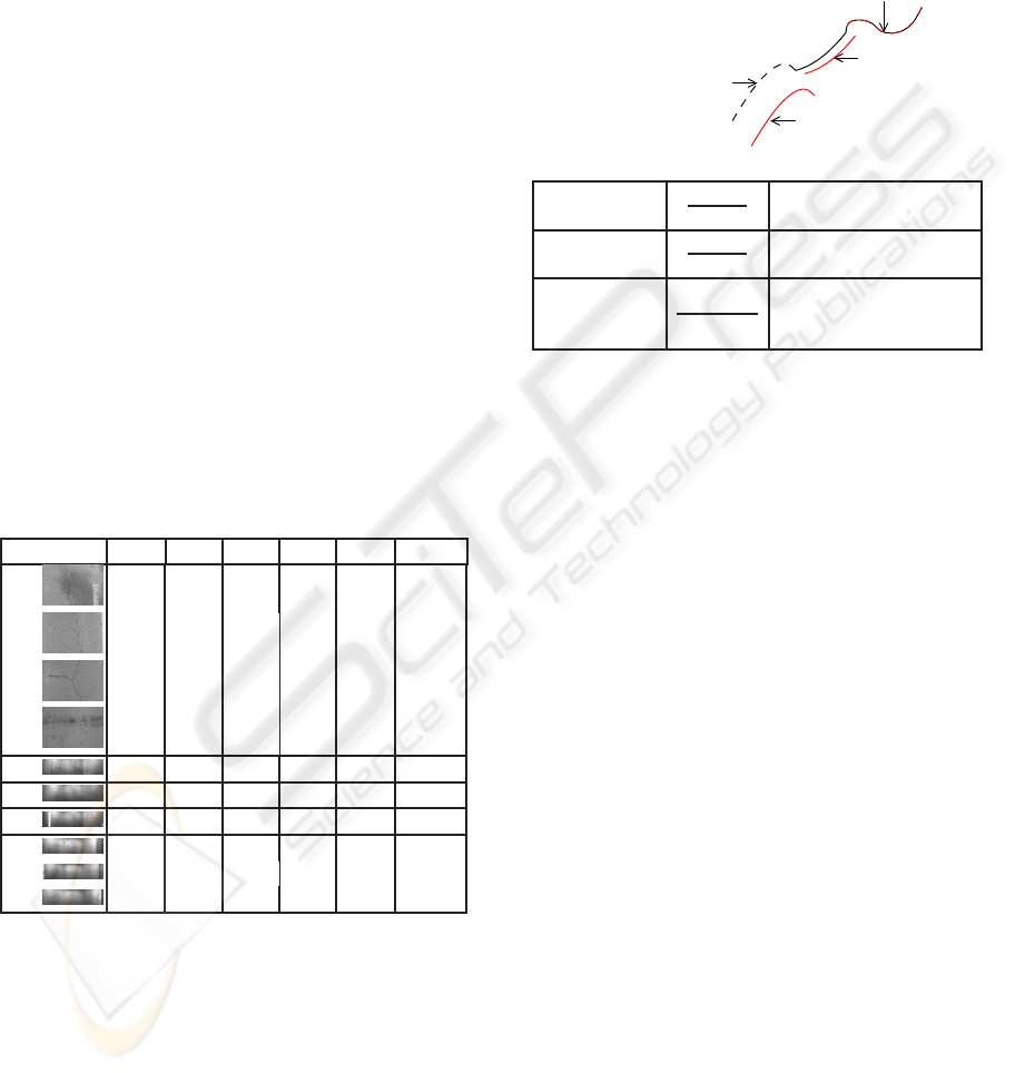
4.3 Evaluation Criteria
In this section, we introduce how the reference seg-
mentation and the estimated segmentation are com-
pared. In Figure 5, we present common evaluation
criteria that are used for segmentation evaluation. We
have added the principle of ”accepted” detection that
tolerates a small error on the localization of crack
pixels. This criterion is needed because perfect de-
tection seems, for the moment, difficult to reach, see
the results in Table 3, that illustrate this aspect. In
consequence, these ”accepted” pixels have been in-
cluded in the estimation of the similarity coefficient
or DICE. The threshold for accepted pixels equals 0
for synthetic images whereas it depends on the mean
distances, see D. in table 3, for the real images.
True positives (TP)
Positives (P)
Accepted
False positives (FP)
False Negatives (FN)
True negatives (TN)
Sensitivity
TP
TP+FN
Proportion of good
detections
Specificity
TN
TN+FP
Proportion of
non-detected pixels
Similarity
coefficient or
Dice similarity
2TP
FN+T P+P
Ratio between good
detections and
non-detections
Figure 5: Evaluation criteria – In this figure, it corresponds
to two simulated segmentations of the same crack: the black
one is manual (or the reference) and the red one is esti-
mated. The goal is to evaluate the quality of the estimated
segmentation, that corresponds to the Positives (P). All the
non-selected pixels that do not correspond to the crack are
called the True Negatives (TN). Piece of crack with the two
colors (red and black) are the correct detections or True Pos-
itives (TP). In the table, the criteria are resumed and in this
work, we have used the DICE because this coefficient well
represents what we want to measure: the quality of the de-
tection against the percentage of the crack that is detected,
or, how to reduce false detections and to increase the den-
sity.
5 EXPERIMENTAL RESULTS
For the proposed method, we want to determine, first,
how to fix the different parameters, second, the pre-
processing steps that are necessary, and, finally, which
variant is the most efficient. In consequence, we have
tested different:
• Parameter values – The weights α
1
, equation (7),
and α
2
, equation (9), are tested from 0 to 1 with a
step of 0.1.
• Pre-processings – These pre-processings have
been experimented to reduce noises induced by
texture, to increase the contrast of the defect and,
to reduce the light halo in some images (like the
last six ones presented in Table 3):
1. Threshold – Each pixel over a given threshold
is replaced by the local average gray levels.
VISAPP 2010 - International Conference on Computer Vision Theory and Applications
86
2. Smoothing – A 3×3 mean filter is applied.
3. Erosion – An erosion with a square structuring
element of size 3×3 is applied.
4. Restoration – It tries to combine the ad-
vantages of all the previous methods in three
steps: histogram equalization, thresholding
(like Threshold), and erosion (like Erosion).
• Algorithm variants – Four variants are compared:
1. Init – This is the initial method proposed
in (Subirats et al., 2006).
2. Gaus – This variant considers the crack as a
Gaussian function, see section 3.2.
3. InMM – This is the initial version with an im-
provement of the Markov model (new defini-
tion of the sites and of the potential function),
see section 3.3.
4. GaMM – This is the Gaus version with the new
Markov model.
• Comparison – We have compared this method
with a method based on morphological tools and
that is quite similar to (Tanaka and Uematsu,
1998) noted Morph.
5.1 Parameter Influence
Among the results, two conclusions can be done. For
each variant and each pre-processing, the weights be-
tween the term for adapted filtering and the term for
the Markovian modelling should be the same, see
equation (7), i.e. α
1
= 0.5. However, when more
weight is given to adapted filtering , the quality of the
results is lower than when more weight is given to the
Markovian segmentation. It means that in this kind
of application, the geometric information is more re-
liable than the photometric one and it seems coherent
with the difficulties of the acquisition.
For the new Markov model, we have noticed that the
results are the best when the weights are the same be-
tween the orientation term and the distance term, see
equation (9), i.e. α
2
= 0.5. However, better results are
obtained when the weight of the orientation is greater
than the distance one instead of the reverse.
5.2 Pre-processing
These tests have been done with real images, be-
cause, a priori, synthetic images do not need pre-
processings. The results are given by:
Init Gaus InMM GaMM
Restoration Restoration Threshold Erosion
However, for the four first images (acquired with
lighting conditions more comfortable than the light-
ing conditions of the next 6 ones), the pre-processing
is not significant for increasing the quality of the re-
sults. Moreover, with the new Markov model, the pre-
processing step increases a little the quality.
Init
Gaus
InMM
GaMM
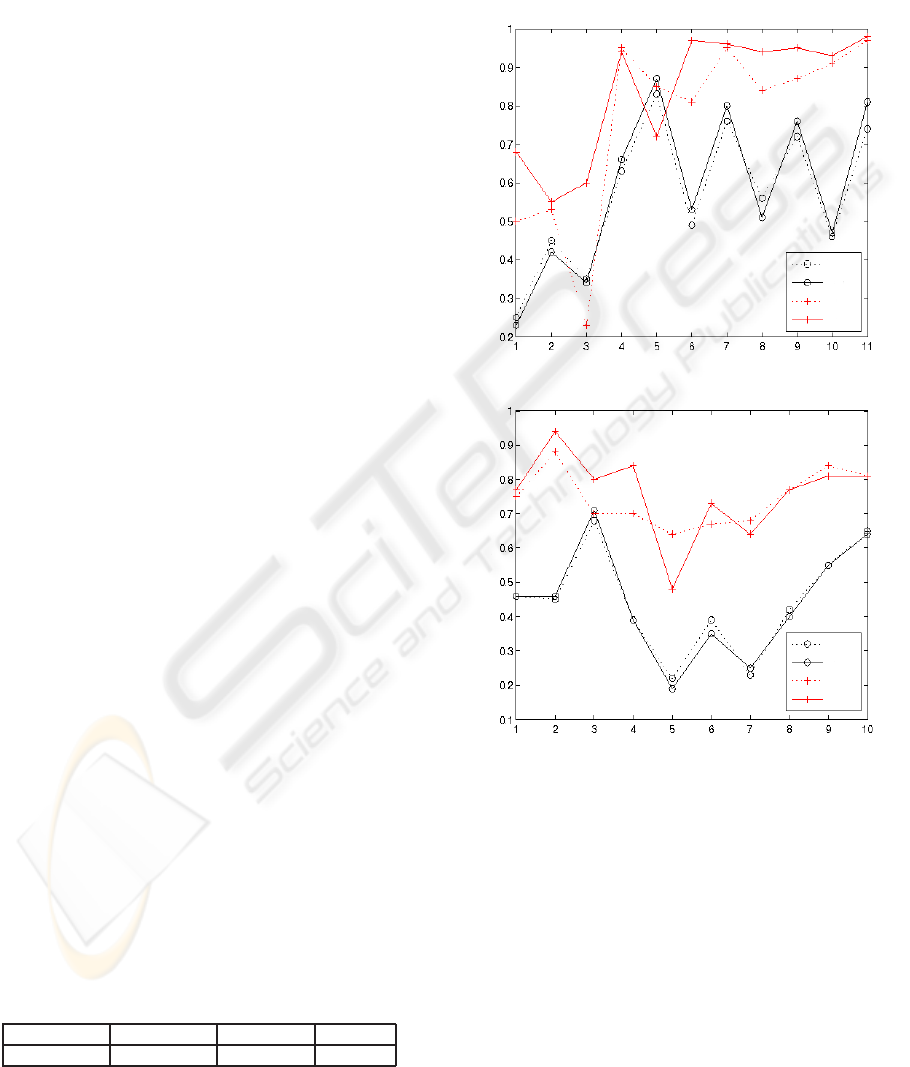
Similarity coefficient
Synthetic images
GaMM
InMM
Gaus
Init
Similarity coefficient
Real images
Figure 6: Variation of the similarity coefficient, see fig-
ure 5 – The first graph shows the results for synthetic im-
ages (the 3 first ones are obtained from real images with
simulated defect) and the second graph presents the results
with real images. Good performances of methods InMM
and GaMM can be noticed.
5.3 Variants
The results are separated in two cases: with synthetic
images and with real images. In Figure 6, the evolu-
tion of the similarity coefficient, or DICE, for the 11
synthetic images and the 10 real images is presented.
With synthetic images, GaMM is clearly the best for
most of the images. However, for one image (the
ROAD CRACK EXTRACTIONWITH ADAPTED FILTERING AND MARKOV MODEL-BASED SEGMENTATION -
Introduction and Validation
87
GaMM
Morph
Similarity coefficient
Real images
Mean
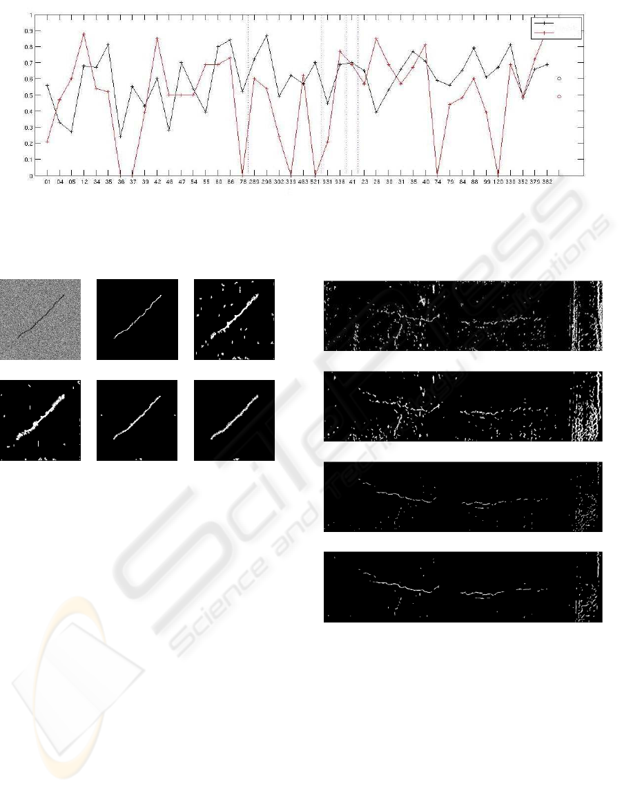
Figure 9: Comparison with Morph – The dotted lines illustrate the five different kinds of images tested. For the first one (that
corresponds to real images with good illumination), the results are mixed whereas for the other ones, GaMM is the best.
Image Ground truth Init
Gaus InMM GaMM
Figure 7: Segmentation results (synthetic images presented
in Figure 4) – These are the results obtained with the four
variants and it shows how GaMM gives the clearest result.
We can also notice the good result of InMM.
fifth), the results are worse than with Gaus but they
are still correct (DICE=0.72). On the contrary, for the
most difficult images (the 3 first ones that contain a
real road background), GaMM obtains acceptable re-
sults (DICE > 0.5) whereas the other methods are not
efficient at all. An illustration is given in Figure 7: it
shows how GaMM can reduce false detections.
The results with real images, see graph (b) in Fig-
ure 6, are coherent with those obtained with synthetic
images. The new Markov model allows the best im-
provements, compared to the initial method Init. The
method GaMM obtains the best results, except on few
images, see an example in figure 8, where InMM is
the best. However, GaMM gives results that are quite
similar and the differences are not significant.
Init
Gaus
InMM
GaMM
Figure 8: Segmentation results (real images) – These are the
results obtained with the real images presented in figure 4.
Method InMM obtains the clearest detection (i.e. with less
false detection) but we can also noticed the good quality of
the detection map with GaMM.
5.4 Complementary Dataset and
Comparison
Finally, we have compared the result of GaMM on
each of the complementary dataset (32 images) with
the results obtained with a classic method based
on morphological tools, like (Tanaka and Uematsu,
1998). The mean DICE is 0.6 with GaMM whereas
VISAPP 2010 - International Conference on Computer Vision Theory and Applications
88
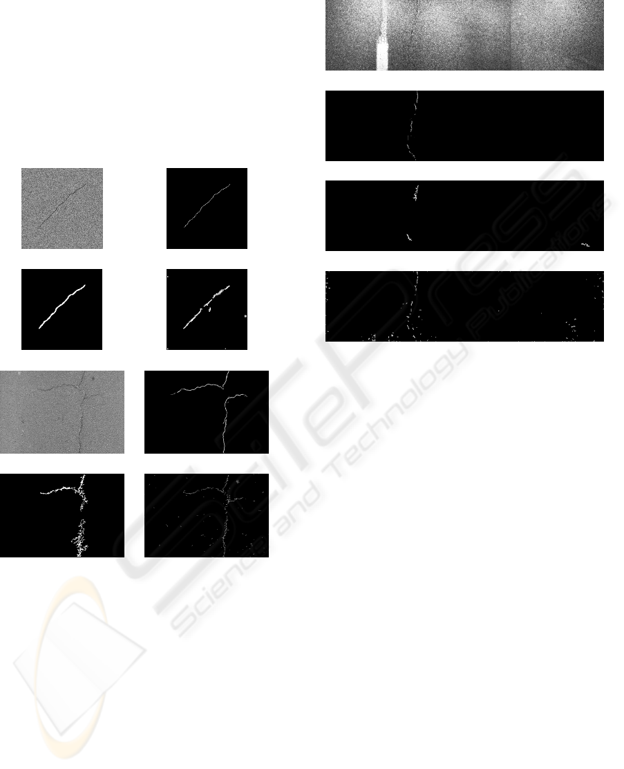
it is 0.49 with the Morphology method, see Figure 9.
It shows how this new method outperforms this kind
of method. However, if we compare image per image,
the results show that in 50% of the cases GaMM is the
best, see illustrations of these results in Figures 10 and
11. More precisely, it seems more performant with
Ambiguous images, whereas the Morphology method
is the best with Reliable images, see § ”Complemen-
tary dataset”.
Synthetic image ”Ground truth”
segmentation
Morph FaMM
Real image Reference segmentation
Morph FaMM
Figure 10: Differences between Morph and GaMM – Ex-
amples with synthetic and real images. Morph outperforms
GaMM with simple synthetic images whereas GaMM gives
better detection with real images.
6 CONCLUSIONS
In a first time, we have introduced new methods for
the detection of road cracks. In a second time, we
have presented a new evaluation and comparison pro-
tocol for automatic detection of road cracks and the
new methods are validated by this protocol. As far
as we are concerned, we proposed real images with
ground truth for the first time in the community. Our
next work is to propose our ground truth to the com-
munity in order to havea larger comparison. Then, we
want to increase our data set by taking into account
Real image
Reference segmentation
Morph
GaMM
Figure 11: Differences between Morph and GaMM – Ex-
amples with real images acquired on a vehicule. The detec-
tion with GaMM is more complete than with Morph.
the different qualities of road surface or road tex-
ture (because for the moment, each proposed method
seems very dependent on the road texture). Finally,
we want to refine our evaluation criteria by using (Ar-
belaez et al., 2009).
REFERENCES
Acosta, J., Adolfo, L., and Mullen, R. (1992). Low-cost
video image processing system for evaluating pave-
ment surface distress. TRR: Journal of the Transporta-
tion Research Board, 1348:63–72.
Arbelaez, P., Fowlkes, C., and Malik, J. (2009). From con-
tours to regions: An empirical evaluation. In Com-
puter Vision and Pattern Recognition. To appear.
Augereau, B., Tremblais, B., Khoudeir, M., and Legeay, V.
(2001). A differential approach for fissures detection
on road surface images. In International Conference
on Quality Control by Artificial Vision.
Bray, J., Verma, B., Li, X., and He, W. (2006). A neural
nework based technique for automatic classification
of road cracks. In International Joint Conference on
Neural Networks, pages 907–912.
Chambon, S., Subirats, P., and Dumoulin, J. (2009). Intro-
duction of a wavelet transform based on 2d matched
filter in a markov random field for fine structure ex-
traction: Application on road crack detection. In
IS&T/SPIE Electronic Imaging - Image Processing:
Machine Vision Applications II.
ROAD CRACK EXTRACTIONWITH ADAPTED FILTERING AND MARKOV MODEL-BASED SEGMENTATION -
Introduction and Validation
89

Cheng, H., Chen, J., Glazier, C., and Hu, Y. (1999). Novel
approach to pavement cracking detection based on
fuzzy set theory. Journal of Computing in Civil En-
gineering, 13(4):270–280.
Chou, J., O’Neill, W., and Cheng, H. (1995). Pavement
distress evaluation using fuzzy logic and moment in-
variants. TRR: Journal of the Transportation Research
Board, 1505:39–46.
Delagnes, P. and Barba, D. (1995). A markov random field
for rectilinear structure extraction in pavement distress
image analysis. In International Conference on Image
Processing, volume 1, pages 446–449.
Elbehiery, H., Hefnawy, A., and Elewa, M. (2005). Sur-
face defects detection for ceramic tiles using image
processing and morphological techniques. Proceed-
ings of World Academy of Science, Engineering and
Technology (PWASET), 5:158–162.
Fukuhara, T., Terada, K., Nagao, M., Kasahara, A., and
Ichihashi, S. (1990). Automatic pavement-distress-
survey system. Journal of Transportation Engineer-
ing, 116(3):280–286.
Iyer, S. and Sinha, S. (2005). A robust approach for auto-
matic detection and segmentation of cracks in under-
ground pipeline images. Image and Vision Computing,
23(10):921–933.
Kaseko, M. and Ritchie, S. (1993). A neural network-based
methodology for pavement crack detection and clas-
sification. Transportation Research Part C: Emerging
Technologies information, 1(1):275–291.
Koutsopoulos, H. and Downey, A. (1993). Primitive-based
classification of pavement cracking images. Journal
of Transportation Engineering, 119(3):402–418.
Lee, H. and Oshima, H. (1994). New Crack-Imaging Proce-
dure Using Spatial Autocorrelation Function. Journal
of Transportation Engineering, 120(2):206–228.
Petrou, M., Kittler, J., and Song, K. (1996). Automatic sur-
face crack detection on textured materials. Journal of
Materials Processing Technology, 56(1–4):158–167.
Ritchie, S., Kaseko, M., and Bavarian, B. (1991). Develop-
ment of an intelligent system for automated pavement
evaluation. TRR: Journal of the Transportation Re-
search Board, 1311:112–119.
Schmidt, B. (2003). Automated pavement cracking assess-
ment equipment – state of the art. Technical Report
320, Surface Characteristics Technical Committee of
the World Road Association (PIARC).
Song, K., Petrou, M., and Kittler, J. (1992). Wigner based
crack detection in textured images. In International
Conference on Image Processing and its Applications,
pages 315–318.
Subirats, P., Fabre, O., Dumoulin, J., Legeay, V., and Barba,
D. (2006). Automation of pavement surface crack de-
tection with a matched filtering to define the mother
wavelet function used. In European Signal Process-
ing Conference, EUSIPCO.
Tanaka, N. and Uematsu, K. (1998). A crack detection
method in road surface images using morphology. In
Machine Vision Applications, pages 154–157.
Wang, K., Li, G., and Gong, W. (2007). Wavelet-based
pavement distress image edge detection with ” trous”
algorithm. In Transportation Research Record, An-
nual Meeting, volume 2024, pages 73–81.
Zhou, J., Huang, P., and Chiang, F. (2005). Wavelet-based
pavement distress classification. TRR: Journal of the
Transportation Research Board, 1940:89–98.
VISAPP 2010 - International Conference on Computer Vision Theory and Applications
90
