
SHADOW MODELING AND DETECTION FOR ROBUST
FOREGROUND SEGMENTATION IN HIGHWAY SCENARIOS
Katherine Batista, Rui Caseiro and Jorge Batista
Institute of Systems and Robotics, DEEC-FCTUC, University of Coimbra, Portugal
Keywords:
Foreground segmentation, Shadow modelling and detection, Traffic surveillance.
Abstract:
This paper presents a method to automatically model and detect shadows on highway surveillance scenarios.
This approach uses a cascade of two classifiers. The first stage of this method uses a weak classifier to ascertain
the color information of possibly shadowed pixels which will be used by the second stage of this method
(strong classifier). The weak classifier estimates the Color Normalized Cross-Correlation (CNCC) and the
color information of the pixels identified as shadow, will be used to build or update multi-layered statistical
shadow models of the RGB appearance of shadow. These models will then be used, by the strong classifier,
to correctly distinguish shadow. To prevent misclassifications from corrupting the results of both classifiers,
spatial dependencies are also taken into account. For this purpose, nonparametric kernel density estimators in
a pyramidal decomposition (PKDE), as well as, Markov Random Fields (MRF) were independently employed.
This technique is being used in a real outdoor traffic surveillance system in order to minimize the effects of
cast vehicle shadows as well as shadows induced by illumination changes. Several results are presented in this
paper to prove its effectiveness and the advantages of applying spatial contextualization methods to the weak
and strong classifiers.
1 INTRODUCTION
Advances in camera technology as well as in scien-
tific areas such as computer vision have lead to the
development of efficient and robust real time traffic
surveillance systems. In this sort of systems, the pre-
cise detection of moving objects is essential. Gen-
erally, most foreground segmentation processes (e.g.
(Zhong and Sclaroff, 2003)) are sensitive to illumina-
tion changes or cast vehicle shadows which can lead
to faulty detections which seriously reduces the effi-
ciency of other dependent processes. More precisely,
cast vehicle shadows can significantly increase the
detected vehicle’s area and lead to its merging with
nearby vehicles. This fact gravely affects the outcome
of any tracking or vehicle counting systems used in
traffic surveillance. Illumination changes, induced by
clouds or camera auto gain control processes can also
generate false positives.
To overcome these problems, several methods have
been developed where some are based on the use of
color (e.g. (Cucchiara et al., 2003) or (Horprasert
et al., 1999)), brightness, reflectance and geometry
information to identify shadowed pixels. In (Cuc-
chiara et al., 2003) shadows are identified by assum-
ing that the difference of the hue and saturation com-
ponents, between the pixel and corresponding back-
ground pixel, change within certain limits. Nonethe-
less, this technique is not flexible, seeing as it requires
the prior definition of parameters which are not adapt-
able to illumination changes and are not constant for
different scenarios. The authors in (Prati et al., 2003)
also refer that this method presents low robustness
in noisy scenarios. T. Horprasert (Horprasert et al.,
1999) analyze the pixel’s normalized brightness and
normalized chromaticity distortions in the RGB color
space and classifies a pixel as shadow using a set of
thresholds. An automatic method is presented to es-
timate these limits, nonetheless, it is computationally
too expensive to be used in a real time traffic surveil-
lance system. Cavallaro (Cavallaro et al., 2005) also
analyze pixel color information, yet in order to over-
come the previously referred problems, combines this
information with spatial constraints based on edge de-
tection. However, this method doesn’t remove shad-
ows whose edge pixels are adjacent to objects and
background pixels without the use of an heuristic
analysis of a temporal shadow tracking procedure.
Other approaches use statistical models to learn and
describe the appearance of cast shadow. For instance,
Liu (Liu et al., 2007) use information obtained from
a color based classifier and employ GMM (Gaussian
Mixture Models) to model shadowed pixels in the
HSV color space. To improve the classifier, they use
148
Batista K., Caseiro R. and Batista J. (2010).
SHADOW MODELING AND DETECTION FOR ROBUST FOREGROUND SEGMENTATION IN HIGHWAY SCENARIOS.
In Proceedings of the International Conference on Computer Vision Theory and Applications, pages 148-157
DOI: 10.5220/0002823401480157
Copyright
c
SciTePress

local region level information to update these mod-
els. Brisson (Martel Brisson and Zaccarin, 2007) also
use pixel color information in the YUV color space
to build a Gaussian mixture shadow model (GMSM).
Nevertheless, seeing as the approach is pixel-based,
the obtained model’s accuracy is dependent on the
color-based classifier’s results throughout time. In
(Huang and Chen, 2008) shadows are identified by
building pixel-based local region shadow models us-
ing GMMs. A global model is also estimated and used
to update the local region models when movement is
rare. The background, foreground and shadow mod-
els are built into a MRF energy function. However,
this method’s weak classifier which provides infor-
mation for the learning of cast shadow, requires the
definition of several parameters that are not adaptable
to illumination changes.
On the other hand, Porikli (Porikli and Thornton,
2005) models shadows by multivariate Gaussians us-
ing RGB color information provided by a pre-filter.
This approach does not require color space transfor-
mation and, seeing as it uses multiple independent
layers to model each shadow pixel, it is more flexible
than the standard GMMs approach to model shadow.
The shadow models are achieved using color informa-
tion provided by a pre-filter that evaluates color vari-
ation such as in (Horprasert et al., 1999). Shadow
pixels are distinguished using these models and mis-
classification are corrected using shadow flow, which
once again is a color-based analysis. One of the main
drawbacks of this method, is the fact that it does not
perform any sort of spatial contextualization of the
pixel’s label. Therefore, foreground pixels which pos-
sess similar color information to modeled shadow are
misclassified.
The method here presented overcomes this flaw by
considering that a pixel’s label is influenced by its
neighboring pixel labels. In a general matter, this
method is composed by a cascade of two classifiers.
To the results of these classifiers, spatial contextual-
ization is induced to correct misclassifications. The
first classifier is a weak classifier, which purpose is
analyzing every segmented foreground pixel and de-
termining whether a pixel is possibly shadow by mea-
suring the similarity between color and texture of
the foreground and corresponding background. This
is done by estimating the Color Normalized Cross-
Correlation (CNCC). This information is used to
build or update statistical models that describe the
RGB appearance of shadow pixels. These multi-
layered pixel-based models are used by the second
classifier (strong classifier) to identify cast shadows.
Nonetheless, erroneous classifications may seriously
compromise the foreground segmentation process. To
minimize the number of misclassifications, the pixel’s
neighboring labels are taken into account. To do so,
two distinct and independent approaches were imple-
mented and compared. One, consists on a pyramidal
decomposition of kernel density estimators (PKDE),
which has as main goal ascertaining probabilistic rep-
resentations of the surrounding pixel labels to im-
prove the results given by the pre-filter. Another tech-
nique also analyzes the spatial label dependencies us-
ing a Markov Random Field (MRF) energy function
which is minimized by the graph cut algorithm.
2 WEAK SHADOW CLASSIFIER
The weak classifier evaluates the segmented fore-
ground pixels to determine whether a pixel is a possi-
ble shadow pixel. The main goal of this classifier is
not to detect shadows accurately, but to filter out some
impossible shadow pixels. The results of this classi-
fier will be used further on by the strong classifier.
The approach here presented estimates the CNCC be-
tween each segmented pixel I
t
and the corresponding
background pixel Bp
t
(see subsection 2.1). To im-
prove the results of this classifier, two distinct tech-
niques were independently applied and compared.
One, uses a PKDE method (presented in subsection
5.1), while another method ascertains the pixel’s la-
bel by using a MRF approach (presented in subsec-
tion 5.2). A quantitative and qualitative analysis of
the results of these two techniques can be found in
subsection 6.1.
2.1 Color Normalized
Cross-Correlation (CNCC)
This classifier measures the similarity of color and
texture between foreground and background, by es-
timating the CNCC (Grest et al., 2003). More pre-
cisely, a pixel is classified as shadow if its texture
is correlated with the corresponding texture of Bp(t).
In order to estimate the CNCC, the brightness infor-
mation is split from the color values, which is done
by representing the pixel’s color in the bi-conic HSL
space (Grest et al., 2003) (see Figure 1.(a)). To mea-
sure the similarity, the correlation between both can
be estimated by projecting the RGB color vector onto
the chromatic HS plane in order to calculate the Eu-
clidean values of hue (h) and saturation (s). This al-
lows the estimation of the scalar product between the
referred pixels (h,s,L) which is proportional to their
correlation. This is quite simple to understand, see-
ing as if they have similar hues (small angle between
SHADOW MODELING AND DETECTION FOR ROBUST FOREGROUND SEGMENTATION IN HIGHWAY
SCENARIOS
149

Figure 1: (a) Representation of the hue and saturation com-
ponents of the HSL color space. (b) Chromatic plane of the
hsL color space (
~
c
a
and
~
c
b
represent the projection of two
color pixels on this plane).
them) and high saturations, the resulting correlation
will be high (see Figure 1.(b)).
Hence, being c
F
and c
B
the color vectors, in the
hsL space, of a foreground and background pixel at
(x,y), the CNCC is estimated over a window M ×N
surrounding those pixels, using the following equa-
tion:
CNCC =
∑
i j
(c
F
xy
•c
B
xy
) −MN
L
F
.L
B
√
VAR
F
VAR
B
; (1)
where,
VAR
k
= (
∑
i j
(c
k
xy
•c
k
xy
) −MNL
k
2
), (2)
and L
F
is the average intensity of the
foreground pixels inside that window,
k ∈ {F( f oreground),B(background)} and
(c
F
xy
• c
B
xy
) = (h
F
i j
,s
F
i j
) ◦ (h
B
i j
,s
B
i j
) + L
F
i j
L
B
i j
, where
the operator ◦ represents the scalar product.
1
For
gray-level pixels, the CNCC will present similar
values to the normalized cross correlation (NCC).
The resulting values of CNCC lie within [0...1], which
can be interpreted as probabilistic measurements, and
the higher they present themselves, the more likely
the pixel is a shadowed pixel. Consequently, a pixel
can be identified as shadow if these values are larger
than a given threshold. Several examples of results of
this procedure are presented in Figure 2.
3 SHADOW MODELING
Shadow pixels can be distinguished by using statisti-
cal models of their RGB appearance. Basically, each
image pixel possesses multiple layers, where each
one of these, represent a different shadow appearance
for that pixel. In this section, a method proposed in
(Porikli and Thornton, 2005), is described to achieve
these shadow models. The process becomes more dis-
criminative the larger the number of layers. However,
1
The negative values are set to zero.
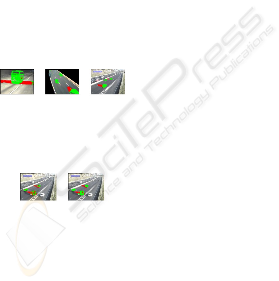
Figure 2: Results of the CNCC weak classifier (red=shadow,
green=foreground).
seeing as this technique is meant to be applied in a real
time system, a large number of layers may compro-
mise the system’s framerate. Thus, we chose to use
three layers seeing as these proved sufficient to statis-
tically describe the color information of shadow. Each
one of these layers can be represented by a multivari-
ate Gaussian distribution corresponding to each color
channel. In other words, for every given pixel, three
layers are estimated, where for each one of these lay-
ers, each RGB channel is modeled by a Gaussian dis-
tribution. To build or update a layer at a given time t,
this method uses the RGB information (x = [r, g,b]) of
a pixel identified as shadow by the weak shadow clas-
sifier. More precisely, to update a layer this method
performs recursive Bayesian estimation using this in-
formation (Porikli and Thornton, 2005). Assuming
the layer follows a normal-inverse-Wishart distribu-
tion, this update can be done using the following ex-
pressions:
υ
t
= υ
t−1
+ n; κ
t
= κ
t−1
+ n; (3)
θ
t
= θ
t−1
κ
t−1
κ
t−1
+ n
+ ¯x
n
κ
t−1
+ n
(4)
Λ
t
= Λ
t−1
+ Σ
n
i=1
(x
i
− ¯x))(x
i
− ¯x))
T
+
+n
κ
t−1
κ
t
( ¯x −θ
t−1
)( ¯x −θ
t−1
)
T
(5)
Σ
t
= (υ
t
−4)
−1
Λ
t
(6)
where, v
t
and Λ
t
are the degrees of freedom and scale
matrix for inverse Wishart distribution, θ
t
the mean,
Σ
t
the covariance and κ
t−1
the number of prior obser-
vations. When the update is performed at each time
frame (i.e. n = 1), the mean of the new samples,
¯x, becomes the pixel’s color information x. These
parameters are re-estimated when a layer is updated
and they describe the pixel’s appearance by combin-
ing the prior information with the new color informa-
tion. When each layer is initialized, the following pa-
rameters are assumed (Porikli and Tuzel, 2005): κ
0
=
10; υ
0
= 10; θ
0
= x
0
; Λ
0
= (υ
0
−4)16
2
I; where I is
a three dimensional identity matrix.
Each layer has also associated a confidence mea-
surement, given by: C =
κ
3
t
(υ
t
−2)
4
(υ
t
−4)|Λ
t
|
, which decreases
with larger variances. This parameter is used in the
layer update algorithm, by sorting the three different
VISAPP 2010 - International Conference on Computer Vision Theory and Applications
150
Algorithm 1: Layer update algorithm.
Input:
1. All pixels identified as foreground;
2. L
i
= different layers (i = 1,..., NU M LAY ERS);
for All pixels identified as foreground: do
1. x = [r, g,b] = pixel identified as shadow by the
weak shadow classifier;
2. Sort layers L
i
(θ
t−1
,Σ
t−1
,υ
t−1
...) according to
confidence measurements.
3. for i ≤ NUM LAY ERS do
(a) Estimate Mahalanobis distance:
d
i
= (x −θ
t−1,i
)
T
Σ
−1
t−1,i
(x −θ
t−1,i
);
(b) if
(Sample x in 99% con f idence interval)
• Update layer L
i
model parameters
(eq. 3
4, 5 and 6);
• Analyze next Pixel x;
else
• Decrease the number of observations:
κ
t
= κ
t−1
−n;
endif
end
4. if No layer updated :
Delete layer L with lowest confidence
measurement and initialize new layer with
new sample and new initial parameters.
endif
end
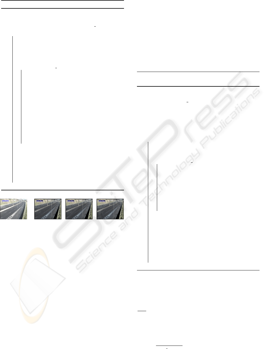
(a) (b) (c) (d)
Figure 3: Background image represented in (a) and the cor-
responding shadow models (ordered from most confident to
least confident (b) to (d)).
layers according to their variances. The layer updat-
ing process is recapitulated in algorithm 1. Figure 3
shows several examples of different shadow models
for a shadowy scenario.
4 SHADOW /FOREGROUND
SEGMENTATION
Foreground pixels are those that are not identified as
background or shadow. The process used to estimate
the background model is not exploited in this paper,
however for more details see (Monteiro et al., 2008).
Having statistically modeled the color appearance of
shadow it is possible to correctly identify the shadow
and true foreground pixels. To do so, the different
shadow layers are sorted accordingly to their confi-
dence measurements and the Mahalanobis distance is
calculated between the pixel’s color and each layer.
Unlike (Porikli and Thornton, 2005), a pixel is not
immediately labelled as shadow if its color informa-
tion lies within the 99% confidence interval of one of
the shadow model layers. This would lead to erro-
neous classifications due to noisy less confident lay-
ers.
Algorithm 2: Shadow classifier algorithm
(Strong Classifier).
Input:
1. L
i
= different shadow layers
(i = 1, ...,NUM LAY ERS);
2. C
min
=Minimum normalized confidence
(threshold);
3. C
∑
min
=Minimum sum of normalized confidence
(threshold);
for All pixels identified as foreground (x = [r, g,b])
do
1. Sort layers L
i
(θ
t−1
,Σ
t−1
,υ
t−1
...) according to
confidence measurements.
2. for i ≤ NUM LAY ERS do
(a) Estimate Mahalanobis distance;
(b) if (x in 99% con fidence interval)
• Normalize the L
i
confidence measurement: C
norm
i
.
• Re-estimate the layer’s sum of
normalized confidence:
C
sum
= C
sum
+C
norm
i
endif
end
3. if ( The layer’s C
norm
i
≥C
min
and C
sum
≥C
∑
min
)
• Pixel classified as shadow.
endif
4. if (Above conditions not satis fied f or no L
i
):
• Pixel classified as foreground.
endif
end
The method here presented avoids labeling as
shadow, pixels that lie within the confidence inter-
val of low confident shadow models. To do so,
each pixel’s layer confidence is normalized (C
norm
i
=
C
i
∑
i
Ci
) and the sum of normalized confidence mea-
surements of model layers with which the sample is
within the 99% confidence interval C
∑
norm
is esti-
mated. If one of these values is lower than two thresh-
olds (i.e. C
norm
i
< C
min
or C
∑
norm
< C
∑
min
, where
C
min
=
1
NUM LAY ERS
and the default C
∑
norm
= 0.5),
then the pixel is not labeled as shadow. This is done
mainly to avoid noisy less confident models from in-
SHADOW MODELING AND DETECTION FOR ROBUST FOREGROUND SEGMENTATION IN HIGHWAY
SCENARIOS
151

ducing erroneous classifications in the segmentation
process. In subsection 6.2 a quantitative analysis is
presented to prove the benefits of introducing these
thresholds (C
min
and C
∑
min
) in this procedure.
Figure 4: (a) Captured image. (b) Most confident shadow
model. (c) Results of the strong classifier.
Vehicle pixels which possess similar color infor-
mation as the shadow models can be mislabelled as
shadow (which can be seen in Figure 4.(c)). To over-
come this drawback, spatial context can be introduced
into this final classification.
5 SPATIAL
CONTEXTUALIZATION
METHODS
By using the pixel’s neighboring label information it
is possible to minimize the number of wrongly classi-
fied pixels. For this purpose, two distinct techniques
were independently employed and compared. One,
uses a PKDE approach (presented in subsection 5.1),
while another method ascertains the pixel’s label by
using a MRF approach (presented in subsection 5.2).
A quantitative and qualitative analysis of the results
of these two techniques can be found in subsection
6.1 and 6.2.
5.1 Pyramidal Decomposition of
Nonparametric Kernel Density
Estimators (PKDE)
The main goal of this method, is to use statistical rep-
resentations of the surrounding pixel labels to correct
erroneous classifications. Having to chose a model
and estimate the distribution parameters is avoided us-
ing nonparametric kernel density estimators (KDE).
Therefore, the distribution’s probability density func-
tion (pdf) can be given by:
p(z) =
1
N
N
∑
i=1
K
h
(z −z
i
) (7)
where, N represents the number of data points and
K
h
is a kernel function with bandwidth h. Choosing
a Gaussian kernel function, the density model can be
achieved by placing a Gaussian over each data point
and adding up the contributions over the whole data
set and normalizing it by dividing this result by the
number of data points (Bishop, 2006), which gives:
p(z) =
1
N
N
∑
i=1
1
(2πh
2
)
1/2
e
−kz−z
i
k
2
2h
2
(8)
Given the fact we are statistically modeling a
pixel’s classification based on its neighboring infor-
mation, the pdf is estimated for a two dimensional
domain space and therefore z becomes z = [x y]. The
resulting two dimensional kernel density model can
then be represented by:
p(z) =
1
N
N
∑
i=1
1
2π(detΣ)
1/2
e
−
1
2
(
[z−z
i
]
T
Σ
−1
[z−z
i
]
)
(9)
where, Σ is the covariance matrix.
By estimating the pdf functions over a M by M
window surrounding the pixel (N = M × M), the
pixel’s label is ascertained. The choice of an appro-
priate kernel function’s bandwidth, h is rather tricky.
If it is too small the kernel density model will be un-
dersmoothed but, on the other hand, if it is too large it
will become over-smoothed. Several automatic band-
width selector methods have been developed through-
out the years, such as MISE (mean integrated square
error) or AMISE (asymptotic MISE) driven meth-
ods (Wand and Jones, 1994). Oversmoothing, least
squares cross-validation, biased cross-validation or
plug-in methods are several examples of AMISE
bandwidth estimator techniques. These methods are
computationally too expensive for real time systems
or require the specification of a pilot bandwidth (plug-
in methods). Nonetheless, simpler methods have
emerged, such as the balloon estimator (Mittal and
Paragios, 2004), where the bandwidth is calculated in
function of the distance from the point to the nearest
data point. However, this method is subject to discon-
tinuities and integration at infinity problems. Another
strategy, known as sample point estimator, calculates
the bandwidth in function of the sample points (Mit-
tal and Paragios, 2004). However, in the method here
proposed, the bandwidth is obtained using a proce-
dure similar to the one proposed in (Mittal and Para-
gios, 2004), and is calculated as the covariance of the
data within the M ×M window (h = Σ). By doing this,
areas with larger uncertainty will be given less weigh-
tage in the pdf function. To minimize the influence of
the size of this M ×M window, a pyramidal image
structure is used, where multi-scaled subsampling is
preformed on the probabilistic data. It is important to
state that the KDE’s bandwidth and probabilities are
calculated for each level of the pyramidal structure in
order to prevent over or under smoothing. The proba-
bilities of a pixel being shadow or foreground are then
VISAPP 2010 - International Conference on Computer Vision Theory and Applications
152
analyzed in a logarithmic scale and the pixel’s label is
finally ascertained.
5.1.1 PKDE Applied to the Results of the Weak
Classifier
Using the CNCC classifier’s results, a pixel can be
identified as shadow when the estimated CNCC is
larger than a given threshold. This threshold can
be empirically set accordingly to the desired shadow
detection rate, i.e. a high threshold will sub-detect
shadow, while a low one will over detect it. However,
threshold driven classifiers are bound to lead to mis-
classifications, such as the ones represented in Fig-
ure 2. To prevent these erroneous classifications from
corrupting the statistical models, the pixel spatial de-
pendencies are analyzed. The result of applying the
PKDE technique to the results of the CNCC weak
classifier are exemplified in Figure 5.
Figure 5: Examples of this weak classifier’s
(CNCC+PKDE) results.
5.1.2 PKDE Applied to the Results of the Strong
Classifier
To improve the results of the strong classifier, the
PKDE (presented in subsection 5.1) was employed.
Figure 6 shows an example of the outcome produced
by this method.
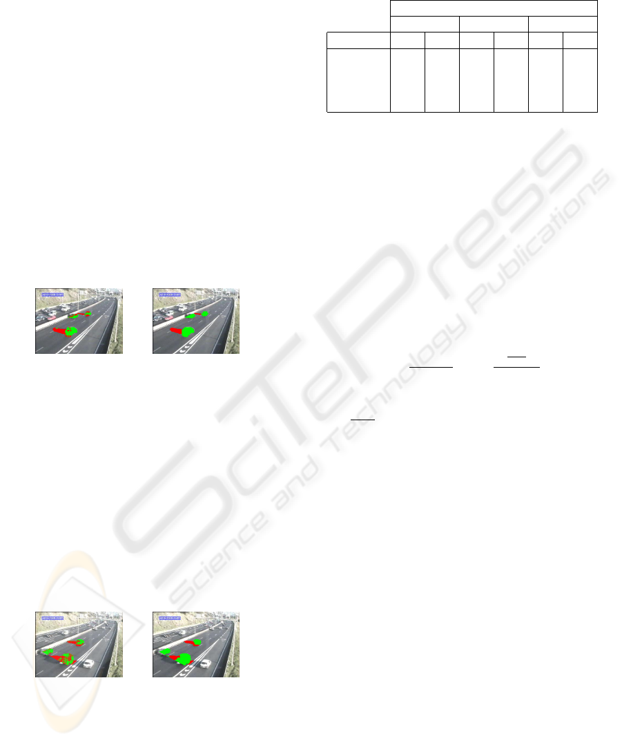
Figure 6: (a) Strong classifier Results. (b) PKDE applied to
the strong classifier results.
5.2 Markov Random Fields (MRF)
Segmentation is a typical vision problem that can
be naturally expressed in terms of energy minimiza-
tion. More specifically, problems that require the es-
timation of spatially varying quantity (intensity, tex-
ture) from noisy measurements, can be formulated
in a Bayesian framework using MRF. Spatial con-
text is an important constraint when making decisions
about a pixel’s label, i.e., a pixel’s label is not inde-
pendent of the pixels neighborhood labels. So, in-
stead of using only likelihood information of mod-
els, MAP (maximum a posteriori)-MRF framework
provides a convenient prior for modelling this spa-
tial interaction. This fact allows a global inference
to be made, using local information, since labels con-
ditional independence rarely exists between proximal
sites. The objective is to assign a binary label l
p
from
the set l
p
∈
{
f oreground,shadow
}
to each of the sites
p ∈ P, where P is the set of segmented pixels, and
L =
{
l
p
|p ∈ P
}
is the global labelling field of random
variables (or configuration of the field). The goal is to
find a L configuration, which minimize a energy func-
tion. In our case the function considered belongs to
F
2
class of energy functions, defined in (Kolmogorov
and Zabih, 2004) as a sum of function of up to two bi-
nary variables at a time. Seeing as it satisfies the con-
ditions proposed in (Kolmogorov and Zabih, 2004)
the optimization of L can be achivied by finding the
minimum cut of a capacitated graph. First order MRF
energy function can be decomposed as follows:
E(L) =
∑
p∈P
[D
p
(l
p
) +
∑
q∈N
p
V
p,q
(l
p
,l
q
)]
(10)
where D
p
(l
p
) is the term derived from the ob-
served data that measures the cost of assigning the
label l
p
to the pixel p (evaluates the likelihood of each
pixel belonging to one of the two classes), V
p,q
(l
p
,l
q
)
measures the cost of assigning the labels l
p
, l
q
to
the adjacent pixeis p, q, and is used to impose spa-
tial smoothness (spatial coherence of labels throught
a pairwise interaction MRF prior, by penalizing dis-
continuities between neighboring pixels), and N
p
is
the set of interacting pairs of pixeis (eight-connected
neighboring). In a real time system, the computa-
tion time is a crucial factor, Greig (Greig et al., 1989)
showed that the MAP solution of a two label pairwise
MRF can be efficiently obtained in polynomial time
by finding the st-mincut on the equivalent graph, pro-
viding an exact global optimial solution. The prior
takes the form of the Ising model, a particular case of
the generalized Potts model, for two label problems.
The piecewise constant smoothness prior is used to
stress spatial context, by assigning penalties for la-
bel discontinuities between neighboring pixels. The
penalty used does not depend on the assigned labels,
as long as they are different, and is spatially invariant.
The data cost term D
p
(l
p
), is defined as the negative
log likelihood of a pixel p belonging to foreground or
shadow class. In the following sections, we will show
how to determine these likelihoods, when MRF is ap-
plied to the weak or to the strong classifier. Graph
cut techniques from combinatorial optimization can
be used to find the global minimum for a multidi-
mensional energy function. MAP estimate of a MRF
can be obtained by solving a multiway minimum cut
problem on a graph. The minimum s/t cut prob-
lem can be solved by finding a maximum flow from
SHADOW MODELING AND DETECTION FOR ROBUST FOREGROUND SEGMENTATION IN HIGHWAY
SCENARIOS
153
the source s to the sink t (Boykov and Kolmogorov,
2004), so energy function of equation 10 can be effi-
ciently minimized by the graph cut algorithms. The
minimum cut of the graph can be computed through
a variety of approaches, like the Ford-Fulkerson al-
gorithm (Ford and Fulkerson, 1962), but in our case
we performed the cut using the min-cut/maxflow al-
gorithm, based on augmenting paths formulated by
Kolmogorov (Boykov and Kolmogorov, 2004).
5.2.1 MRF Applied to the Results of the Weak
Classifier
The CNCC weak classifier provides results that can
be taken as independent probabilistic measurements
for the pixel’s label. Thus, these results can be used
as the likelihood of a pixel’s label in the MRF energy
function. In this case, the procedure does not require
the definition of thresholds. Figure 7 shows several
examples of the application of this technique.
Figure 7: (a) Weak CNCC Classifier results. (b) Weak Clas-
sifier + MRF results.
5.2.2 MRF Applied to the Results of the Strong
Classifier
To apply the MRF approach, the sum of normal-
ized confidences of layers with which the sample lies
within the confidence interval, is used as the likeli-
hood of the pixel’s label. The higher this sum presents
itself, the more likely the pixel is indeed a shadow
pixel and therefore, it provides a spatial independent
probabilistic measurement for that pixel’s label. Fig-
ure 8 shows several results of applying this techniques
to the results of the model driven shadow classifier.
Figure 8: (a) Strong Classifier results. (b) Strong Classifier
+ MRF results.
6 RESULTS
To analyze the effectiveness of this method, ground
truth shadow and foreground pixels were identified
on a sequence of 450 frames of a highway scenario.
Table 1: η and ξ rates of several weak classifier methods for
three different thresholds.
Thresholds
0.3 0.5 0.7
Methods η ξ η ξ η ξ
CNCC 88.0 74.0 76.7 90.6 54.3 97.9
CNCC +KDE 88.1 75.6 76.8 91.3 53.9 98.2
CNCC +PKDE 83.6 88.9 71.6 97.6 41.6 99.7
CNCC +MRF 78.3 96.6 78.3 96.6 78.3 96.6
Not all vehicles were identified, only the ones on the
lanes closest to the surveillance camera. In this sec-
tion several results of applying these methods to this
sequence are presented. To evaluate the accurateness
of each method, the metrics presented in (Prati et al.,
2003) are used to estimate the rates of false positives
and negatives. More precisely, to measure the number
of false negatives (i.e. shadow pixels wrongly clas-
sified as foreground) the shadow detection rate η is
estimated and to measure the false positives (i.e. fore-
ground pixels classified as shadow) the shadow dis-
crimination rate ξ is calculated, using the following
expressions:
η =
T P
S
T P
S
+FN
S
ξ =
T P
F
T P
F
+FN
F
(11)
where, T P is the number of true positives (pixels cor-
rectly classified), FN is the number of false nega-
tives, T P
F
is the number of ground-truth points of
the foreground objects minus the number of points
detected as shadows, but belonging to foreground ob-
jects, while F and S represent foreground and shadow,
respectively.
This section is composed of two main parts, where the
first presents a quantitative and qualitative analysis of
the performance of the weak shadow classifier. In the
second part, the same analysis is performed for the
results obtained by the overall process for foreground
segmentation and shadow detection.
6.1 Weak Shadow Classifier Results
In this subsection, the performance of four indepen-
dent weak shadow classifier methods are compared.
The first is the result of estimating each pixel’s CNCC
and classifying it as shadow if this value is above a
pre-defined threshold. The second method employs a
kernel density estimator (KDE) to the results of this
classifier, while the third applies the PKDE approach.
The last uses the estimated CNCC in a MRF frame-
work. To analyze the outcome of these methods, three
different thresholds where applied and their perfor-
mances compared.
VISAPP 2010 - International Conference on Computer Vision Theory and Applications
154
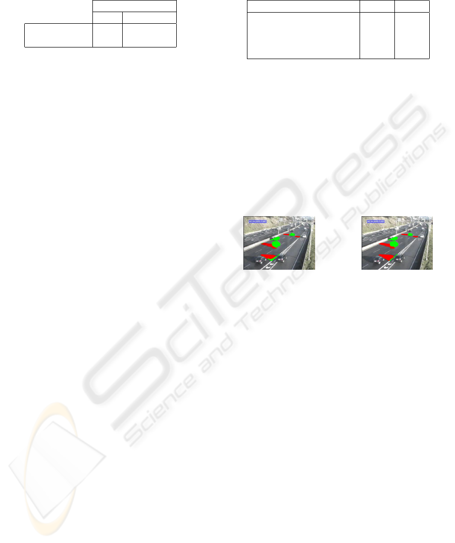
Table 2: η and ξ rates obtained by taking or not into account
thresholds (C
min
and C
∑
min
).
Strong Classifier
η ξ
No thresholds 94.4 69.4
Thresholds 87.7 80.1
The weak classifier’s main goal is to correctly
identify as many shadow pixels as possible. There-
fore, the aim is to achieve a high shadow discrim-
ination rate, ξ, seeing as it indicates a low number
of false positives. The shadow detection rate, η, is
as well important seeing as if it is low, the shadow
models will take too long to converge. Analyzing
the results obtained for the threshold driven methods
(CNCC, KDE, PKDE) presented in Table 1, it is pos-
sible to see a clear improvement using the KDE ap-
proach and an even higher ξ using the PKDE tech-
nique. However, the shadow detection rate is clearly
low in this last method (41.59%). It is important
to state that these methods are threshold driven and
their performances are clearly dependent of the de-
fined threshold. Therefore, the wisest choice for this
weak classifier is the MRF approach, seeing as its effi-
ciency does not rely on the chosen threshold and its ξ
and η are quite high (96.6% and 78.3% respectively).
6.2 Foreground/Shadow Segmentation
Results
The main goal of a good shadow classifier is too
achieve high ξ and η. The results presented in this
section were achieved throughout the final 100 frames
of the test sequence, seeing as the first 350 where
used to estimate the multi-layered shadow models.
This was done in order to correctly evaluate the im-
pact of using these models in the shadow classifica-
tion process. Due to all the reasons explained in sub-
section 6.1, the chosen weak classifier is the MRF
approach. Table 2 presents the results obtained by
the foreground segmentation process (Strong Classi-
fier which corresponds to algorithm 2) when thresh-
olds (C
min
and C
∑
min
) are taken into account.
The performance of this classifier improves sig-
nificantly by introducing these thresholds, seeing as ξ
increases, which indicates a lower percentage of fore-
ground pixels identified as shadow. The shadow de-
tection rate η decreases slightly but is, nevertheless,
still quite high (87.7%).
Introducing spatial context to the results of this strong
classifier, several misclassifications are going to be
corrected, namely, false positives induced by pixels
belonging to vehicles that present similar color infor-
mation as the shadow models. Table 6.3 presents the
Table 3: η and ξ rates for the Strong Classifier methods
using the last 100 frames.
Methods η ξ
Strong Classifier 87.68 77.06
Strong Classifier+KDE 89.10 79.65
Strong Classifier+PKDE 83.01 94.34
Strong Classifier+MRF 91.91 84.50
results of independently applying the KDE technique,
as well as the PKDE estimator and yet, the MRF ap-
proach to the results of the strong classifier. Examin-
ing this table, it is possible to see that employing the
PKDE and MRF techniques to the results of the strong
classifier, ξ increases and therefore, the percentage
of false positives is reduced significantly. Comparing
more thoroughly the results of both these methods, it
is possible to see that the PKDE procedure presents
a higher ξ (lower percentage of false positives) but
a lower η when compared with the MRF approach.
Figure 9 shows an example of this behavior.
(a) PKDE approach (b) MRF approach
Figure 9: Results of Strong Classifier associated with
PKDE and MRF approaches.
However, both methods present good detection
rates and can be efficiently applied to induce spatial
context to the results given by the strong classifier.
Nonetheless, a qualitative analysis of both methods
indicates that the MRF approach preforms a more ac-
curate spatial contextualization than the PKDE tech-
nique.
To support this claim, a quantitative interpretation
was made by applying the Distance Transform to im-
ages containing the ground truth and classified fore-
ground and shadow pixels. The distance transform
sets each image pixel as the distance to the nearest
boundary pixel. Therefore false positives located in
the outmost regions of the blob will possess lower
distance transform values seeing as these are closer
to the nearest boundary pixel. By comparing these
values and the one obtained for the ground truth, it
is possible to ascertain an estimate on the errors of
the spatial contextualization made by each method.
Table 6.4 presents the shadow detection and shadow
discrimination rates obtained using the equations in
expression 11, but considering the distance transform
values instead of the actual number of true positives
or false negatives. As expected, η and ξ of the MRF
SHADOW MODELING AND DETECTION FOR ROBUST FOREGROUND SEGMENTATION IN HIGHWAY
SCENARIOS
155
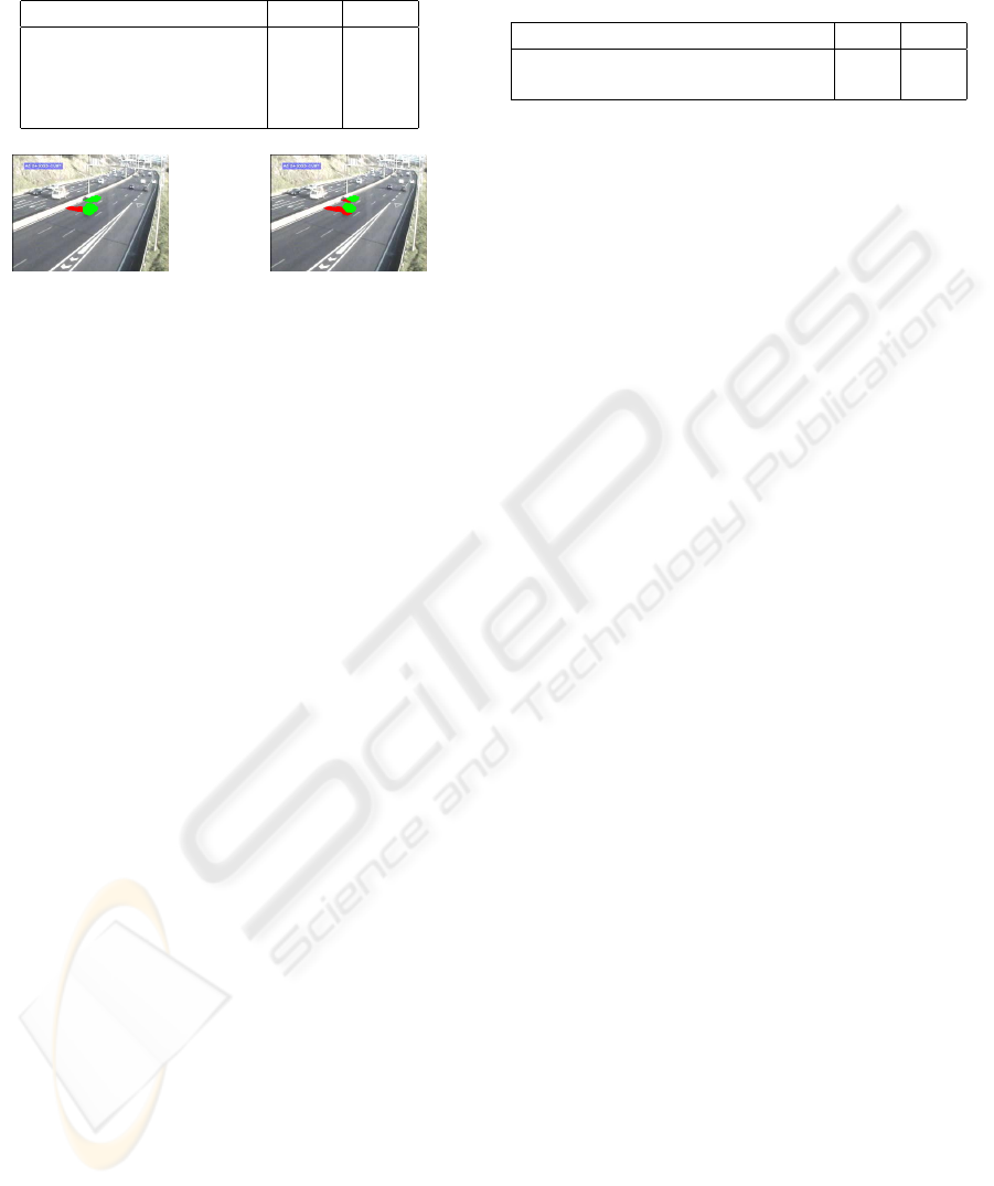
Table 4: Spatial context efficiency analysis of the strong
classifier techniques (using the Distance Transform).
Methods η ξ
Strong Classifier 93.05 77.17
Strong Classifier+KDE 94.27 80.30
Strong Classifier+PKDE 88.36 95.69
Strong Classifier+MRF 95.90 93.95
(a) (b)
Figure 10: (a) Weak classifier + MRF results. (b) Strong
Classifier + MRF results.
technique are quite high.
Nevertheless, the PKDE is computationally less
expensive than the MRF process, which is an impor-
tant factor in a real time surveillance system. Looking
at the results given by the weak classifier (present in
Table 1), one question may arise: what is the need of
statistical shadow models, seeing as this classifier al-
ready presents acceptable results? Yet, it is possible
to see that using a strong classifier aided by the MRF
technique, clearly improves the shadow detection rate
η, which means that the percentage of false negatives
is significantly reduced. Although the number of false
positives increased, these are mainly located on the
borders of the blobs and do not significantly deterio-
rate the vehicle segmentation process. An example of
this behavior is shown in Figure 10 where, due to the
non identification of shadow, it is possible to see that
the leftmost vehicle’s area is remarkably larger, when
employing only the weak classifier.
The Distance transform was applied to carry out
the same spatial context analysis performed previ-
ously. Looking at the results presented in Table 6.5,
it is possible to conclude that this technique identifies
shadow more accurately, seeing as, in a global mat-
ter, the weak classifier identifies less shadow which
can lead to discontinuous blobs or blobs with consid-
erably larger areas.
7 CONCLUSIONS
This paper presented an automatic method to iden-
tify cast vehicle shadow. This method pre-identifies
shadow pixels and uses their color information to de-
velop multi-layered statistical models that describe
the RGB appearance of shadow. These shadow
Table 5: Spatial context efficiency analysis of the strong
classifier and weak classifier techniques (using the Distance
Transform).
Methods η ξ
Weak Classifier + MRF approach 90.40 98.20
Strong Classifier + MRF approach 95.90 93.95
models were used to correctly label shadow pixels.
To overcome misclassification, two independent pro-
cesses (PKDE and MRF), that induce spatial con-
text to the results of the classifiers, were employed
and compared. The PKDE technique presented ac-
ceptable results and is computationally less expen-
sive than the MRF approach. Nevertheless, its re-
sults proved to be slightly poorer than the MRF ap-
proach, which is also threshold invariant and there-
fore a more reliable approach. In order to employ this
technique in a real time highway surveillance system,
multiprocessing systems were used in its implementa-
tion. The method was thoroughly tested on a highway
scenario sequence, where the ground truth foreground
and shadow pixels were identified. The obtained re-
sults are quite satisfactory (91.91% shadow detection
rate and 84.5% shadow discrimination rate).
REFERENCES
Bishop, C. M. (2006). Pattern Recognition in Machine
Learning. Springer.
Boykov, Y. and Kolmogorov, V. (2004). An experi-
mental comparison of min-cut/max- flow algorithms
for energy minimization in vision. Pattern Analy-
sis and Machine Intelligence, IEEE Transactions on,
26(9):1124–1137.
Cavallaro, A., Salvador, E., and Ebrahimi, T. (2005).
Shadow-aware object-based video processing. IEEE
Proceedings - Vision, Image and Signal Processing,
152(4):398–406.
Cucchiara, R., Grana, C., Piccardi, M., and Prati, A. (2003).
Detecting moving objects, ghosts, and shadows in
video streams. IEEE Transactions on Pattern Anal-
ysis and Machine Intelligence, 25(10):1337–1342.
Ford, L. R. and Fulkerson, D. R. (1962). Flows in Networks.
Princeton University Press.
Greig, D. M., Porteous, B. T., and Seheult, A. H. (1989).
Exact maximum a posteriori estimation for binary im-
ages. Royal Statistical Soc., Series B, 51:271–279.
Grest, D., michael Frahm, J., and Koch, R. (2003). A color
similarity measure for robust shadow removal in real
time. In Proc. of Vision, Modeling, and Visualization
(VMV).
Horprasert, T., Harwood, D., and Davis, L. S. (1999). A sta-
tistical approach for real-time robust background sub-
traction and shadow detection. In ICCV Frame-Rate
WS.
VISAPP 2010 - International Conference on Computer Vision Theory and Applications
156

Huang, J. B. and Chen, C. S. (2008). Learning Mov-
ing Cast Shadows for Foreground Detection. In The
Eighth International Workshop on Visual Surveillance
- VS2008, Marseille France. Graeme Jones and Tieniu
Tan and Steve Maybank and Dimitrios Makris.
Kolmogorov, V. and Zabih, R. (2004). What energy func-
tions can be minimized via graph cuts? IEEE Trans-
actions on Pattern Analysis and Machine Intelligence,
26:147–159.
Liu, Z., Huang, K., Tan, T., and Wang, L. (2007). Cast
shadow removal combining local and global fea-
tures. Computer Vision and Pattern Recognition,
IEEE Computer Society Conference on, 0:1–8.
Martel Brisson, N. and Zaccarin, A. (2007). Learning
and removing cast shadows through a multidistribu-
tion approach. IEEE Trans. Pattern Anal. Mach. In-
tell., 29(7):1133–1146.
Mittal, A. and Paragios, N. (2004). Motion-based back-
ground subtraction using adaptive kernel density esti-
mation. volume 2, pages II–302–II–309 Vol.2.
Monteiro, G., Marcos, J., Ribeiro, M., and Batista, J.
(2008). Robust segmentation for outdoor traffic
surveillance. In ICIP, pages 2652–2655.
Porikli, F. and Thornton, J. (2005). Shadow flow: A recur-
sive method to learn moving cast shadows. Computer
Vision, IEEE International Conference on, 1:891–
898.
Porikli, F. and Tuzel, O. (2005). Bayesian background mod-
eling for foreground detection. In ACM International
Workshop on Video Surveillance and Sensor Networks
(VSSN), pages 55–28.
Prati, A., Mikic, I., Trivedi, M. M., and Cucchiara, R.
(2003). Detecting moving shadows: Algorithms and
evaluation. IEEE Transactions on Pattern Analysis
and Machine Intelligence, 25(7):918–923.
Wand, M. P. and Jones, M. C. (1994). Kernel Smoothing
(Monographs on Statistics and Applied Probability).
Chapman & Hall/CRC.
Zhong, J. and Sclaroff, S. (2003). Segmenting foreground
objects from a dynamic textured background via a ro-
bust kalman filter. Computer Vision, IEEE Interna-
tional Conference on, 1:44.
SHADOW MODELING AND DETECTION FOR ROBUST FOREGROUND SEGMENTATION IN HIGHWAY
SCENARIOS
157
