
BELIEF PROPAGATION IN SPATIOTEMPORAL GRAPH
TOPOLOGIES FOR THE ANALYSIS OF IMAGE SEQUENCES
Volker Willert
Control Theory and Robotics Lab, TU Darmstadt, Landgraf-Georg-Str. 4, 64283 Darmstadt, Germany
Julian Eggert
Cognitive Control Group, Honda Research Institute, Carl-Legien-Str. 30, 63073 Offenbach, Germany
Keywords:
Early Vision, Dynamical Vision, Belief Propagation, MRF, DBN, Denoising.
Abstract:
Belief Propagation (BP) is an efficient approximate inference technique both for Markov Random Fields
(MRF) and Dynamic Bayesian Networks (DBN). 2DMRFs provide a unified framework for early vision prob-
lems that are based on static image observations. 3D MRFs are suggested to cope with dynamic image data.
To the contrary, DBNs are far less used for dynamic low level vision problems even though they represent se-
quences of state variables and hence are suitable to process image sequences with temporally changing visual
information. In this paper, we propose a 3D DBN topology for dynamic visual processing with a product of
potentials as transition probabilities. We derive an efficient update rule for this 3D DBN topology that unrolls
loopy BP for a 2D MRF over time and compare it to update rules for conventional 3D MRF topologies. The
advantages of the 3D DBN are discussed in terms of memory consumptions, costs, convergence and online
applicability. To evaluate the performance of infering visual information from dynamic visual observations,
we show examples for image sequence denoising that achieve MRF-like accuracy on real world data.
1 INTRODUCTION
Probabilistic graphical models like 2D grid-based
Markov Random Fields (Szeliski et al., 2008) com-
bined with approximate inference techniques like Be-
lief Propagation (Pearl, 1988) are successfully used
for several kinds of early vision tasks like image de-
noising, stereo vision and optical flow computation.
The main ability of a MRF is to robustly infer hidden
states of a visual scene like pixel depth or movement
based on local noisy image measurements. The core
of a 2D MRF for low level visual processing is the res-
olution of estimation ambiguities via incorporation of
models describing the spatial context between neigh-
boring pixels. At the moment the vision community
investigates in extending these models to improve ro-
bustness and estimation accuracy (Roth, 2007; Rama-
lingam et al., 2008; Komodakis and Paragios, 2009)
and developsfast approximate inference techniques to
head for realtime applications (Szeliski et al., 2008;
Felzenszwalb and Huttenlocher, 2006; Petersen et al.,
2008). Another important aspect concerning online
visual knowledge extraction is the dynamics of visual
scenes. Hence, temporal changes in the observed vi-
sual data and the fact that future observations cannot
be accessed have to be considered. To keep all the
properties of a 2D MRF but also model a whole se-
quence of images, the 3D MRF was introduced by
(Williams et al., 2005) and has further been investi-
gated by several researchers (Yin and Collins, 2007;
Larsen et al., 2007; Chen and Tang, 2007; Huang et
al., 2008). Here, 2D MRFs like in figure 1 a) that
model the spatial relations within a single time slice
are stacked into a 3D spatiotemporal MRF as shown
in figure 1 b). To impose spatiotemporal constraints
usually each node of the 2D MRF in the current frame
is connected to its four image neighbors and addition-
ally to the nodes with the same grid coordinates in the
previous and next frames. This results in a graph of
cardinality six on which the basic BP algorithm can
be used without modifications (Williams et al., 2005).
Whenever visual observations with moving ob-
jects or taken from a moving camera system are
processed, then the temporal correspondences be-
tween image coordinates of consecutive time slices
are changing (Chen and Tang, 2007; Huang et al.,
117
Willert V. and Eggert J. (2010).
BELIEF PROPAGATION IN SPATIOTEMPORAL GRAPH TOPOLOGIES FOR THE ANALYSIS OF IMAGE SEQUENCES.
In Proceedings of the International Conference on Computer Vision Theory and Applications, pages 117-124
DOI: 10.5220/0002818501170124
Copyright
c
SciTePress

p
pp
p
q
p
q
q
a) b) c)
t − 1t − 1 tt t + 1t + 1
Figure 1: a) A 2D grid-like pairwise MRF with four neighboring nodes (fat black lines) in the Markov blanket of a hidden
Figure 1: a) A 2D grid-like pairwise MRF with four neighboring nodes (fat black lines) in the Markov blanket of a hidden
node p (white circles). b) A 3D grid-like pairwise MRF with 6 nodes in the Markov blanket. c) A 3D DBN with directed links
between spatiotemporal neighboring nodes (5 node Markov blanket) indicated by black arrows (only one connection pattern
is shown for clarity). All observable nodes are omitted.
2008). Hence, knowledge about on which coordinates
is projected the same scene content between two time
slices has to be incorporated into the temporal tran-
sitions. As a correspondence field the optical flow
can be used. This leads to a spatially and temporally
adaptive neighborhood connection between nodes of
consecutive time slices. Since in most cases the op-
tical flow cannot be estimated unambiguously for ev-
ery pixel in an image sequence special care has to be
taken for the integration of such an uncertain corre-
spondence information.
Instead of extending MRFs from a 2D grid to a 3D
grid structure, another class of probabilistic graphical
models could be used to model spatiotemporal depen-
dencies, called Dynamic Bayesian Networks. They
generalize coupled hidden Markov models (HMM)
(Brand, 1997) by representing the hidden state in
terms of state variables with complex interdependen-
cies and are suitable for online filtering and prediction
(Murphy and Weiss, 2001).
The main aim of this paper is to answer the ques-
tion: What kind of connectivity is the most efficient
one if both spatial and temporal information should be
fed into every node of a 3D grid-like graph? The ques-
tion is motivated by finding an efficient solution to
early vision problems with visual observations being
dynamic. To do so, we compare belief propagation
for different MRF graph topologies with DBN graph
topologies. We propose to use a special connectivity
in a 3D DBN topology that allows to come as close as
possible to the basic BP algorithm for MRFs. Hence,
for the 3D DBN we assume the same 3D grid-like
structure as for 3D MRFs but different node connec-
tions.
The main differences between the conventional
3D MRF topology and the proposed 3D DBN topol-
ogy are: (I) The conventional 3D MRF has several
undirected links between neighboring nodes within a
time slice but usually only two temporal neighbors
(see figure 1 b)) for an example with 4 spatial neigh-
bors). (II) The proposed 3D DBN has no undirected
links between neighboring nodes within a time slice
but directed links between one node at current time
and several neighboring nodes of an arbitrary number
from the past time slice (see figure 1 c)) for an exam-
ple with 4 spatiotemporal neighbors).
1
Introducing
a factorised transition probability for DBNs, we are
able to compare BP in 2D MRFs and 3D MRFs to BP
in 3D DBNs. We show that inference in a 3D DBN
with the proposed topology and connectivity is less
memory consuming, less computationally expensive,
and better suited for online filtering than their MRF
counterpart.
To cope with a temporally changing image content
because of moving objects and therefore with tempo-
rally adaptive correspondences between image pixels
of consecutive frames, we use optical flow as a cor-
respondence field for adaptation of the node connec-
tions of the 3D DBN as it was already proposed in
(Chen and Tang, 2007) and (Huang et al., 2008) but
for 3D MRFs.
2 MRF AND DBN DEFINITIONS
For early vision problems usually a pairwise MRF is
used that is based on a 2D grid-like graph structure
as shown in figure 1 a). Following the notation in
(Felzenszwalb and Huttenlocher, 2006), let P be the
set of pixels p ∈ P in an image. Each pixel is assigned
two nodes - one for a hidden random variable x
p
∈ X
and one for an observed random variable y
p
∈ Y . X
denotes a finite set of variable values and Y a finite
1
In principle, the connections and the number of neigh-
boring nodes can vary but we restrict ourselves to equal con-
nection patterns for every node on the image grid.
VISAPP 2010 - International Conference on Computer Vision Theory and Applications
118

set of observations
2
. Further on, let (p,q) ∈ N be
an edge between the hidden random variables x
p
and
x
q
from the set N of all edges in the graph. A hid-
den state X consists of an amount of state variables
{x
p
}
p∈P
for each pixel p and the observation Y com-
prises all pixel observations {y
p
}
p∈P
. The joint dis-
tribution of a pairwise 2D MRF is given by
P(X,Y) =
1
Z
∏
p∈P
φ(x
p
,y
p
)
∏
(p,q)∈N
ψ(x
p
,x
q
), (1)
where φ(x
p
,y
p
) denotes the node potential that de-
fines the similarity between the observed pixel mea-
surement and the hidden labels and ψ(x
p
,x
q
) corre-
sponds to the edge potentials that encode the similar-
ities of spatially neighboring labels. The quantity Z
is a normalization constant, called the partition func-
tion.
Extending the 2D MRF to a 3D MRF leads to
an increase in the number of state variables with an
additional time index t ∈ T for a sequence of T =
(1,2,... ,T) time slices. The hidden and observed
states, X
t
= {x
t
p
}
t∈T
p∈P
and Y
t
= {y
t
p
}
t∈T
p∈P
, are repre-
sented in terms of hidden and observed state variables,
x
t
p
∈ X and y
t
p
∈ Y . This allows for temporally chang-
ing observations. Thus, the joint distribution of a pair-
wise 3D MRF for a sequence of image observations
Y
1:T
is given by
P(X
0:T
,Y
1:T
) =
1
Z
∏
(p,q)∈N
ψ(x
0
p
,x
0
q
) ×
∏
t∈T
∏
p∈P
φ(x
t
p
,y
t
p
)ψ(x
t
p
,x
t−1
p
) ×
∏
(p,q)∈N
ψ(x
t
p
,x
t
q
). (2)
Here, the edge potentials ψ(x
0
p
,x
0
q
) at time t = 0 intro-
duce some initial state conditions.
To transfer the spatiotemporal properties of a 3D
MRF to a 3D DBN, we restrict ourselves to regu-
lar
3
DBNs (Murphy and Weiss, 2001) with a spe-
cial topology like depicted in figure 1 c). The
generative model of a DBN is precisely defined
by the specification of the observation likelihood
P(Y
t
|X
t
) =
∏
p
P(y
t
p
|x
t
p
) and the transition probabil-
ity
4
P(X
t
|X
t−1
) =
∏
p
P(x
t
p
|{x
t−1
q
}) with q ∈ N (p)
2
Without loss of generality, the observations can be dis-
crete or continuous.
3
Within one time slice the hidden and observable nodes
are arranged like the 2D pixel-grid of an image. Directed
connections are only allowed from hidden nodes x
t
p
to ob-
servables y
t
p
at the same time or to neighboring hidden
nodes x
t−1
q
from the past time slice. Intra-slice connections
between neighboring hidden nodes x
t
p
and x
t
q
at the same
time are forbidden.
4
Sometimes also called conditional probability tables.
and N (p) being a neighborhood of grid position p
including a set of neighboring hidden nodes {x
t−1
q
} at
grid positions q in the past time slice. The joint like-
lihood of a DBN up to time T is given by
P(X
0:T
,Y
1:T
) =
∏
p∈P
P(x
0
p
)P(x
1
p
|{x
0
q
}) ×
∏
t∈T
∏
p∈P
P(y
t
p
|x
t
p
)P(x
t
p
|{x
t−1
q
}), (3)
where P(x
0
p
) are the priors of the state variables that
serve as initialisation.
3 BELIEF PROPAGATION
Now, we focus on comparing inference in MRFs and
in DBNs for online applications. The strategy is to
select an approximate inference technique for MRFs
that is closely related to forward filtering in DBNs and
to choose the transition of a DBN such that the differ-
ences between inference on the MRF and the DBN
get as small as possible. This allows to discuss the
advantages of the remaining differences in the infer-
ence algorithms.
3.1 Belief Propagation for a 2D MRF
Using loopy BP in a 2D MRF at each iteration
step n, an approximation for the marginal probabil-
ity P(x
p
,Y) called the belief for each node p can be
computed
b
n
(x
p
) ∝ φ(x
p
,y
p
)
∏
q∈N (p)
m
n
q→p
(x
p
). (4)
Here, m
n
q→p
(x
p
) are the incoming messages to node
p within the spatial neighborhood N (p) where the
proportionality ∝ considers
∑
x
p
m
n
q→p
= 1. Applying
the sum-product algorithm (Bishop, 2006) the mes-
sage update visualised in figure 2 a) is given by
m
n
q→p
(x
p
) ∝
∑
x
q
∈X
ψ(x
p
,x
q
)φ(x
q
,y
q
)
∏
s∈N (q)\p
m
n−1
s→q
(x
q
)
∝
∑
x
q
∈X
ψ(x
p
,x
q
)
b
n−1
(x
q
)
m
n−1
p→q
(x
q
)
, (5)
where m
n−1
s→q
(x
q
) are the incoming messages to node q
other than p: N (q)\p. For initialisation all messages
are set to be uniform m
0
q→p
= 1, ∀(p,q).
3.2 Belief Propagation for a 3D MRF
For an online application with temporally changing
observations we can apply a forward BP on a 3D MRF
BELIEF PROPAGATION IN SPATIOTEMPORAL GRAPH TOPOLOGIES FOR THE ANALYSIS OF IMAGE
SEQUENCES
119

p
qq
q
p
q
p
q
p
a) b) c)
t − 2 t − 2t − 1 t − 1t t
Figure 2: Message passing schedules for a) a pairwise 2D Markov random field b) a pairwise 3D Markov random field and c)
Figure 2: Message passing schedules for a) a pairwise 2D Markov random field b) a pairwise 3D Markov random field and c)
a 3D DBN. For the 3D DBN the spatiotemporal information flow is not restricted to the five neigbors from past time slice but
can be an arbitrary number of node connections. Observation nodes are omitted for clarity. Hidden nodes being operated on
for a message update are shown white with the message flow indicated by arrows; other hidden nodes are displayed black.
with a message update schedule that does not access
future observations (Yin and Collins, 2007). Now the
forward belief for each node p for each timestep t is
defined as
b
n
(x
t
p
) ∝ φ(x
t
p
,y
t
p
) m
p→p
(x
t
p
)
∏
q∈N (p)
m
n
q→p
(x
t
p
). (6)
The messages have to be updated according to the fol-
lowing defined order if we do not want to go back-
wards in time. First, the messages for the temporal
transition (see figure 2 b)) are calculated as given by
m
q→q
(x
t
q
) ∝
∑
x
t−1
q
∈X
ψ(x
t
q
,x
t−1
q
)φ(x
t−1
q
,y
t−1
q
) ×
m
q→q
(x
t−1
q
)
∏
s∈N (q)
m
n
s→q
(x
t−1
q
)
∝
∑
x
t−1
q
∈X
ψ(x
t
q
,x
t−1
q
)b
n
(x
t−1
q
), (7)
which is recurrent over time t in m
q→q
(x
t
q
) ←
f(m
q→q
(x
t−1
q
))
5
. Second, the spatial messages within
a time slice are calculated (see figure 2 b)) as follows
m
n
q→p
(x
t
p
) ∝
∑
x
t
q
∈X
ψ(x
t
p
,x
t
q
)φ(x
t
q
,y
t
q
) ×
m
q→q
(x
t
q
)
∏
s∈N (q)\p
m
n−1
s→q
(x
t
q
)
∝
∑
x
t
q
∈X
ψ(x
t
p
,x
t
q
)
b
n−1
(x
t
q
)
m
n−1
p→q
(x
t
q
)
, (8)
which are dependent on the temporal transitions
m
q→q
(x
t
q
) and the spatial transitions m
n−1
s→q
(x
t
q
) that
can be iteratively refined along n = 1...N iterations
anew for each time slice t. Here, all the speed-ups
proposed for message passing in 2D MRFs like in
(Felzenszwalb and Huttenlocher, 2006; Tappen and
Freeman, 2003) can be applied.
5
f denotes the function that transfers m
q→q
(x
t−1
q
) to the
next time t.
3.3 Belief Propagation for a 3D DBN
For the forward BP on a 3D DBN we use an ef-
ficient approximate inference algorithm called fac-
torised frontier algorithm (Murphy and Weiss, 2001).
It assumes that the posterior probability P(X
t
|Y
1:t
) :=
∏
p
P(x
t
p
|Y
1:t
) is approximated as a product of
marginals which is equivalent to loopy BP assuming
that the messages coming into a node are indepen-
dent. For inference, we define the observation likeli-
hood as the product of the node potentials used for the
3D MRF
P(Y
t
|X
t
) =
∏
q∈P
P(y
t
p
|x
t
p
) =
∏
p∈P
φ(x
t
p
,y
t
p
), (9)
and the transition as the normalised product of the
edge potentials
P(x
t
p
|{x
t−1
q
}) ∝
∏
q∈N (p)
ψ(x
t
p
,x
t−1
q
), (10)
where ∝ denotes that
∑
x
t
p
P(x
t
p
|{x
t−1
q
}) = 1. It is fur-
ther assumed that every ψ(x
t
p
,x
t−1
q
) is equivalent to
ψ(x
t
p
,x
t−1
p
), ∀q ∈ N (p) of the 3D MRF. With the be-
forehand mentioned assumption of a fully factorised
posterior each factor of the posterior P(x
t
p
|Y
1:t
) is
equivalent to the belief b(x
t
p
) when applying forward
BP on the 3D DBN
P(x
t
p
|Y
1:t
) = b(x
t
p
) ∝ φ(x
t
p
,y
t
p
)
∏
q∈N (p)
m
q→p
(x
t
p
).
(11)
The corresponding forward message update rule (see
figure 2 c)) reads
m
q→p
(x
t
p
) ∝
∑
x
t−1
q
∈X
ψ(x
t
p
,x
t−1
q
)φ(x
t−1
q
,y
t−1
q
) ×
∏
s∈N (q)
m
s→q
(x
t−1
q
)
∝
∑
x
t−1
q
∈X
ψ(x
t
p
,x
t−1
q
)b(x
t−1
q
). (12)
VISAPP 2010 - International Conference on Computer Vision Theory and Applications
120

Inserting the message update (12) into (11) we arrive
at a temporal recurrent belief update
b(x
t
p
) ∝ φ(x
t
p
,y
t
p
)
∏
q∈N (p)
∑
x
t−1
q
ψ(x
t
p
,x
t−1
q
)b(x
t−1
q
),
(13)
which is recurrent over time t only in the beliefs
b(x
t
p
) ← f({b(x
t−1
q
)}). Here, f denotes the function
that transfers past beliefs at time t − 1 to beliefs b(x
t
p
)
at current time t. This is a nice advantage compared
to the belief update in the 3D MRF according to (6)
which is not recurrent over time in the beliefs only.
4 QUALITATIVE COMPARISON
Now the advantages of the recurrent belief update of
the 3D DBN (13) compared to the belief updates of a
2D MRF (4) and a 3D MRF (6) along with the mes-
sage updates are discussed.
Inference. The forward BP in a 3D DBN as pro-
posed in (13) is equivalent to the α-expansion of the
forward-backward-algorithm for Bayesian networks
(Bishop, 2006) as can be seen by the following con-
version
b(x
t
p
) = P(x
t
p
|Y
1:t
)
∝ P(y
t
p
|x
t
p
)
∑
X
t−1
P(x
t
p
|X
t−1
)P(X
t−1
|Y
1:t−1
)
∝ P(y
t
p
|x
t
p
)
∑
X
t−1
∏
q∈N (p)
ψ(x
t
p
,x
t−1
q
)
∏
z∈P
P(x
t−1
z
|Y
1:t−1
)
∝ P(y
t
p
|x
t
p
)
| {z }
φ(x
t
p
,y
t
p
)
∏
q∈N (p)
∑
x
t−1
q
ψ(x
t
p
,x
t−1
q
)P(x
t−1
q
|Y
1:t−1
)
| {z }
b(x
t−1
p
)
×
∑
X
t−1
\x
t−1
q
∏
z6=q
P(x
t−1
z
|Y
1:t−1
)
| {z }
=1
, (14)
assuming the transition probability to be a product of
potentials as defined in (10) and the approximation of
a fully factorised marginal distribution (11) within a
time slice t. Of course, all the derivations also hold for
the max-product algorithm by simply replacing the
marginal sums with the max-operator (Bishop, 2006)
to estimate the most probable sequence of states. Ob-
viously, the DBN update rule (12) looks pretty much
the same as the 2D MRF update rule (5). The only
three differences are that
1. index n is now an iteration through time t and for
each timestep a new state variable x
t
p
is defined,
2. hence the past node x
t−1
s
at position s = p is also
allowed to send a message m
s=p→q
(x
t−1
q
) to con-
tribute to the update of message m
q→p
(x
t
p
) (which
means the belief b(x
t−1
q
) does not have to be di-
vided by the message m
p→q
(x
t−1
q
))
3. and all observations y
t−1
q
are allowed to change
over time.
As a result, the proposed forward filter for the 3D
DBN unrolls the standard loopy BP for a 2D MRF
that iterates n-times within a time slice along the
physical time t and thus can deal with temporally
changing observations. Vice versa, this relation can
be used to define a more approximativebut less mem-
ory consuming BP for 2D MRFs simply by replacing
physical time t in (13) with iteration index n which
reads
b
n
(x
p
) ∝ φ(x
p
,y
p
)
∏
q∈N (p)
∑
x
q
ψ(x
p
,x
q
)b
n−1
(x
q
),
(15)
where the beliefs are initialised equally distributed for
n = 0. To compare it with the standard belief update,
we insert (5) into (4). This leads to
b
n
(x
p
) ∝ φ(x
p
,y
p
)
∏
q∈N (p)
∑
x
q
∈X
ψ(x
p
,x
q
)
b
n−1
(x
q
)
m
n−1
p→q
(x
q
)
,
(16)
which is dependent on the past beliefs {b
n−1
(x
q
)} and
the past messages {m
n−1
p→q
(x
q
)}. The simpler update
rule (15) is much more efficient because it is recursive
in the belief only.
Comparing the belief update of a 3D DBN (13)
with the update of a 3D MRF (6) we have seen in
section 3.2 that (6) is not recurrent in the beliefs only
but is (13). Thus, for the 3D MRF all the messages
have to be stored which is not the case for the belief
update of the 3D DBN.
Memory. Loopy BP methods that do not explic-
itly compute and store messages but directly update
the belief recurrently as in (13) and (15) require
less amount of memory than state-of-the-art mes-
sage passing update rules as in (5) and (7,8). The
space complexity for storing beliefs in (13) and (15)
is P × X . Whereas for storing messages using (5)
or (7,8) the space complexity is P × X × N (p) or
P × X × (N (p) + 1), respectively.
5 QUANTITATIVE COMPARISON
Costs. The time complexity for one message update
step in MRFs increases quadratically in the number
BELIEF PROPAGATION IN SPATIOTEMPORAL GRAPH TOPOLOGIES FOR THE ANALYSIS OF IMAGE
SEQUENCES
121
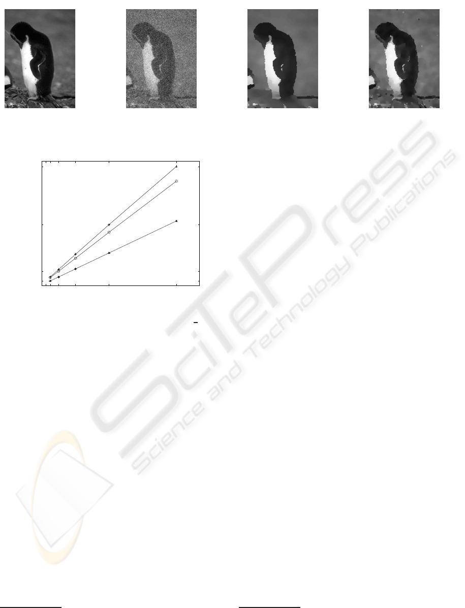
image noisy image denoised image using (16) denoised image using (15)
PSNR = 18.6 PSNR = 25.9 PSNR = 26.8
Figure 3: Denoising results for applying (16) and (15) to the penguin benchmark.
816 32 64 128 256
1
35.1
174.6
666.3
L
C + 3D MRF (7,8)
◦ 2D MRF (15)
∗ 3D DBN (13) or (15)
Figure 4: Costs C for different update rules and label num-
bers L with C = 1 equals a processing time of 0.27
s
u
sec-
onds per update. The y-axis is square-root-scaled because
the time complexity increases quadratically with the num-
ber of labels X .
of state values and linearly in the number of pixels
and messages O (P × X
2
× N ) whereas for the DBN
update the order reduces to O (P ×X
2
). A quantitative
comparisonthat confirms the time complexity is given
in figure 4. Here, the times needed to compute one
update of all beliefs or messages for an image with
120 × 180 pixels for different numbers of labels and
different BP methods are visualized
6
. It confirms the
quadratic increase of the costs with linear increase in
labels and the computational advantage of (13) or (15)
compared to (5) or (7,8).
Accuracy. To compare the accuracy of the differ-
ent BP methods, we start by applying (16) in com-
parison to (15) on the penguin denoising example
(Szeliski et al., 2008). For the denoising test we add
static Gaussian noise with a variance of 30 to the im-
age with a size of 120 × 180 pixels. The state val-
ues x
p
and observables y
p
are intensities with X =
6
The algorithms are implemented in matlab and have
been run on an Intel Core2 2.4GHz with 2GB RAM.
(1,... ,256). For the node potentials we use quadratic
costs φ(x
p
,y
p
) = exp(−l
φ
(x
p
− y
p
)
2
) and for the edge
potentials we use truncated absolute costs ψ(x
p
,x
q
) =
exp(−l
ψ
min(t
ψ
,|x
p
− x
q
|))
7
. Figure 3 shows the de-
noising results after n = 30 iterations for applying
(16) and (15) to the penguin benchmark. The Peak-
Signal-To-Noise-Ratio (PSNR) which quantifies the
denoising quality is slightly better for (15) than for
(16) although the computational effort for (15) is
much less as already shown in Fig. 4.
6 DYNAMIC DENOISING
Temporal Correspondence. If the visual scene
moves, then the temporal pixel correspondences c
t
p
between image coordinates of consecutive time slices
are changing. This requires a spatially adaptive neigh-
borhood N (q+c
t
q
) for the temporal message passing
schedule already proposed in (Chen and Tang, 2007;
Huang et al., 2008). Now, in (7) the temporal mes-
sages m
(q+c
t
q
)→q
(x
t
q
) adapt dependent on the corre-
spondences c
t
q
and in (13) the belief update gets adap-
tive in the product over spatiotemporal neighboring
beliefs q ∈ N (p+ c
t
p
).
To demonstrate the real world applicability of the
proposed BP in 3D DBNs (13) we apply them to solve
an image sequence denoising task and compare the
result to BP in 3D MRFs (7,8). For the 3D MRF,
we restrict the iterations within a time slice (8) to
n = 1 to get a fair comparison to the 3D DBN re-
sults. If the n-iterations are increased the convergence
gets faster per temporal t-iteration but also the com-
putation time increases n-times. Figure 5 shows the
denoising result for BP in a 3D DBN compared to a
3D MRF applied to the car sequence and using opti-
7
The parameters are fixed to −l
φ
= 0.01, −l
ψ
= 0.1,
t
ψ
= 20.
VISAPP 2010 - International Conference on Computer Vision Theory and Applications
122
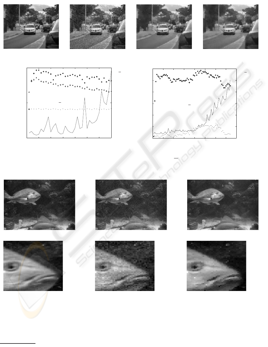
frame 17 noisy frame 17 3D MRF denoising 3D DBN denoising
Figure 5: Denoising results for the car sequence.
0 5 10 15 20 25 30 35
20
25
30
0 5 10 15 20 25 30 35
0
20
40
PSNR
t
E
∗ PSNR DBN denoised
+ PSNR MRF denoised
. . . PSNR noisy
− motion energy
E
(a) Car sequence
0 10 20 30 40 50 60 70 80
27
28
29
30
31
32
33
0 10 20 30 40 50 60 70 80
0
5
10
15
20
25
30
PSNR
t
E
∗ PSNR DBN denoised
. . . PSNR noisy
− motion energy
E
(b) Fish sequence
Figure 6: PSNR and Mean Motion Energy E.
frame 52 noisy frame 52 3D DBN denoising
detail PSNR = 28.1 PSNR = 32.7
Figure 7: Denoising results for the fish sequence.
cal flow for estimating the pixel correspondences c
t
p
8
.
We used the same node and edge potentials as for
8
All sequences and optical flows are taken from
http://people.csail.mit.edu/celiu/motionAnnotation/index.html.
the penguin example but now the noise is a dynamic
additive Gaussian noise with a variance of 16. The
corresponding course of the PSNRs is shown in Fig.
6a. The DBN (∗) always outperforms the denoising
quality of the MRF (+) (the PSNR of the noisy se-
BELIEF PROPAGATION IN SPATIOTEMPORAL GRAPH TOPOLOGIES FOR THE ANALYSIS OF IMAGE
SEQUENCES
123

quence is shown with the dotted line). To judge the
dependency of the denoising quality on the amount of
movements in the sequence also the mean motion en-
ergy E
t
= 1/P
∑
p
||c
t
p
||
2
is plotted. With increasing
motion energy the denoising quality decreases. Fig-
ure 7 shows another denoising example with a detail
for better visual inspection of the results. Although,
the variance of the noise varies between 14 − 16 and
the motion energy increases, the denoising quality
follows quite stable.
We would like to mention that if the number of
intra-time iterations n ≥ 1 is increased it is likely
that the MRF- result could surpass the accuracy of
the DBN but with the disadvantage of increasing the
computing time n-times. Further on, more temporal
neighbors could be used in the MRF, a choice that is
also likely to improve the quality of the MRF-result
but again leads to additional computing time.
7 SUMMARY AND
CONCLUSIONS
We introduce a special 3D DBN topology with an effi-
cient class of transition probabilities as a basic frame-
work for low level vision applications suited for ac-
tive vision systems. It provides promising results in
terms of memory amount, computational costs, and
robustness. Applications for image denoising show
that for static scenes with static noise the proposed
approximate BP achieves similar or better accuracy
for denoising than standard BP in 2D MRFs. For
dynamic scenes an efficient spatiotemporal node con-
nection for a DBN topology is introduced that allows
for fast BP with less memory load than standard 3D
MRF approaches and more accurate denoising results
on noisy real world image sequences.
REFERENCES
Bishop, C. (2006). Pattern Recognition and Machine
Learning. Springer Science+Business Media.
Brand,M. (1997). Coupled hidden markov models for com-
plex action recognition. In Proc. of IEEE Conf. on
CVPR.
Chen, J. and Tang, C. (2007). Spatio-temporal markov ran-
dom field for video denoising. In Proc. of IEEE Conf.
on CVPR.
Felzenszwalb, P. and Huttenlocher, D. (2006). Efficient be-
lief propagation for early vision. Int. J. Comput. Vi-
sion, 70:4154.
Huang, R., Pavlovic, V., and Metaxas, D. (2008). A new
spatio-temporal mrf framework for video-based ob-
ject segmentation. In Proc. of 1st Int. Workshop on
Machine Learning for Vision-based Motion Analysis.
Komodakis, N. and Paragios, N. (2009). Pairwise energies:
Efficient optimization for higher-order mrfs. In Proc.
of IEEE Conf. on CVPR.
Larsen, E., Mordohai, P., Pollefeys, M., and Fuchs, H.
(2007). Temporally consistent reconstruction from
multiple video streams using enhanced belief propa-
gation. In Proc. of IEEE Conf. on CVPR.
Murphy, K. and Weiss, Y. (2001). The factored frontier
algorithm for approximate inference in dbns. In Proc.
of 17th Conf. on Uncertainty in Artificial Intelligence.
Pearl, J. (1988). Probabilistic Reasoning in Intelligent Sys-
tems: Networks of Plausible Inference. Morgan Kauf-
mann.
Petersen, K., Fehr, J., and Burkhardt, H. (2008). Fast gener-
alized belief propagation formap estimation on 2d and
3d grid-like markov random fields. In Proc. of 30th
Conf. of the German Association for Pattern Recogni-
tion.
Ramalingam, S., Kohli, P., Alahari, K., and Torr, P. (2008).
Exact inference in multi-label crfs with higher order
cliques. In Proc. of IEEE Conf. on CVPR.
Roth, S. (2007). High-Order Markov Random Fields for
Low-Level Vision. PhD thesis, Brown University.
Szeliski, R., Zabih, R., Scharstein, D., Veksler, O., Kol-
mogorov, V., Agarwala, A., Tappen, M., and Rother,
C. (2008). A comparative study of energy min-
imization methods for markov random fields with
smoothness-based priors. IEEE Trans. on PAMI,
30:10681080.
Tappen, M. and Freeman, W. (2003). Comparison of graph
cuts with belief propagation for stereo, using identical
mrf parameters. In Proc. of IEEE ICCV.
Williams, O., Isard, M., and MacCormick, J. (2005). Es-
timating disparity and occlusions in stereo video se-
quences. In Proc. of IEEE Conf. on CVPR.
Yin, Z. and Collins, R. (2007). Belief propagation in a 3d
spatio-temporal mrf for moving object detection. In
Proc. of IEEE Conf. on CVPR.
VISAPP 2010 - International Conference on Computer Vision Theory and Applications
124
