
MODELING THE FRAGILE ECONOMIC SITUATIONS
Stasys Girdzijauskas
Vilnius University, Kaunas Faculty of Humanities, Department of Informatics, Muitines str. 8
LT-44280, Kaunas, Lithuania
Andzela Mialik, Ramunas Mackevicius
Vilnius University, Kaunas Faculty of Humanities, Muitines str. 8, LT-44280, Kaunas, Lithuania
Keywords: Modeling of economic situations, Economic bubbles, Logistic model, Predict.
Abstract: The development of the modern society is dependent on its economic growth. In the given logistic theory, a
uniform system of the scientific statements, calculations and estimations has been maintained. An automatic
computer model for fragile economic situations has already been worked out. Yet better results in the
comprehension of the model are achieved when all the calculations are done manually, with the help of the
MS Excel. Therefore the paper introduces the teaching method that might be helpful in understanding how
to operate with the model in a non-automatic way.
1 INTRODUCTION
The world seems to have been enchained by the
constantly appearing financial problems that alarm
both the ordinary people and scientists who get more
and more involved in the analysis of the causes of
the crises. Research is carried out each year with the
goal of discovering the crisis prediction
mechanisms. That is why it is essential to start
teaching the students to understand the causes
determining the fragile economic situations and
show how should be modeled.
Relevance of the Topic.
The difficulties in the
economic crisis prediction, the frequent
misunderstanding of the fundamental basics of the
reasons and development of such crises, as well as
the real possibility of the financial shocks create the
assumptions for an uneven economic development
thus causing an appearance of the threat of social
convulsions.
In 2002–2006, an original theory of the capital
management was worked out at Vilnius University
(Lithuania). It has been discovered that the logistic
growth seems to be based on the idea so well
expressed by an American author Flannery
O'Connor in the very title of her short story
collection "Everything That Rises Must Converge”
(1965). In economics, however, this principle has
started to be applied only recently (Girdzijauskas S.,
Streimikiene D., Dubnikovas M., 2009).
The discussed logistic analysis is based on the
fundamental principles developed in the classical
financial theory. (Merkevicius E. et al., 2007). Based
on the mentioned theory of logistic growth, the
special curricula have been structured, which more
and more often are found as urgent and therefore are
successfully developed. Today, since the consistent
patterns of economics still do astonish the mankind,
the university students of the appropriate study
programs should be taught to recognize and model
various economic situations.
The logistic theory is much more complex than
the classical financial analysis, and no doubt, its
mastery requires the specific resources for learning.
The objective of the paper is to
comprehensively and visually demonstrate the
algorithm of the economic heat and bubble
formation.
The main tasks of the paper are:
• to present how the fragile economic situations
are formed and to give an example,
graphically and comprehensively
demonstrating the process of the bubble
formation;
167
Girdzijauskas S., Mialik A. and Mackevicius R. (2010).
MODELING THE FRAGILE ECONOMIC SITUATIONS.
In Proceedings of the 2nd International Conference on Computer Supported Education, pages 167-170
DOI: 10.5220/0002770401670170
Copyright
c
SciTePress

• to help the students in understanding the
effectiveness of the logistic model in
analyzing the fragile economic situations.
2 LOGISTIC MODELING
The logistic model is applied for the growing
populations. Moreover, it should be stressed that
growth itself is proportional to the size of the same
population and has a determined growth limit. The
paper aims to reveal how the comprehension process
can be simplified by visualizing the modeling
(Girdzijauskas S., Pikturna A., et al., 2008).
In order to employ the principle of logistic
growth in calculations, one should have the general
understanding of the phenomenon of the exponential
change, that may be conveniently expressed by a
differential Equation 1 (Girdzijauskas S., 2006, p.
65).
∫∫
⋅= dtk
K
dK
(1)
here K is accumulated capital (the amount of the
product at the time t); k is the coefficient of
proportionality (constant quantity); K
0
=K(t=0)
(ibid.).
Modeling the growth of the capital on the basis
of this equation, the growth is found to be infinite. In
other words, it is obvious that the equation cannot be
used to predict the long term capital growth
(Girdzijauskas S., 2008).
Already in the 19
th
century, while studying the
alterations in the biological systems, P. F. Verhülst
suggested to add a multiplier to the differential
equation which has the character of a linearly
decreasing function. Let's apply a similar growth-
limiting multiplier to the differential product
alteration equation (Girdzijauskas S., 2006, p. 277):
Kr
K
K
dt
dK
p
⋅⋅
⎟
⎟
⎠
⎞
⎜
⎜
⎝
⎛
−= ln1
(2)
(
)
()
()
11
1
0
0
−++
+⋅⋅
=
n
p
n
p
iKK
iKK
K
(3)
here K
0
is initial capital; K
p
points to potential
capital expressed in the capital amount estimating
units; i is the rate of interest; n is the number of the
periods of accumulation.
The method of the internal rate of return is one of
the essential means in project estimation. When
calculating the internal rate of return by using the
logistic method, it is necessary to know the potential
capital K
p
of each member of the payment chain
(Moskaliova V., Girdzijauskas S., 2006, p. 91). Then
the following equation is worked out:
()
()
0
1
1
0
=
+⋅−+
⋅
+
∑
=
n
j
j
jpj
jp
iKKK
KK
K
.
(4)
The analysis of the logistic net present value of
the money flows and of the internal rate of return
show that the effectiveness of an investment (in
other words, internal return) depends on the degree
of the market filling by the investment capital.
(Girdzijauskas S., Streimikiene D. et al, 2009,
p.267). Thus, the estimation of the growth resources
within the frame of the logistic capital theory turns
to be one of the most important tasks in solving the
problems of rational capital management.
By adapting the particular software tools and
performing the logistic analysis, the economic
bubbles and other economic phenomena that make
the cause of recessions and crises might be
discovered.
For precision, let's explore the heat (growth of
the bubble) model within the following example
table 1:
The investment project is determined to be
realized within 5 years. The net present value (in
complex and logistic percentage) with the rate of
return: a) 10 %; b) 20 % should be calculated as
well as the internal rate of. To perform the logistic
calculations it is necessary to take the following:
K
p
Є[1; ∞) of the conditional monetary unit.
Table 1: Money investment flows.
Year
Monetary flows at the end of the year
Expenses Income Total
0 -1 0 -1
1 -0.5 0 -0.5
2 -0.5 1 0.5
3 -0.5 1 0.5
4 -0.5 1 0.5
5 0 1 1
Total: -3 4 1
Source: worked out by the authors
Let's explore the profitability of an investment in
two ways: (a) by using the complex percentage rule
(when the capacity of the market is unlimited); (b)
by employing the logistic analysis (when the
capacity of the market is limited).
Under the initial condition, we have the
following: K
0
= -1, …, K
5
= 1; i = 8 % (case a)) and
i = 12 % (case b)).
CSEDU 2010 - 2nd International Conference on Computer Supported Education
168
Further steps will show the ordinary or typical
calculations. With the help of the Microsoft Excel
programme it has been discovered that the IRR
(internal rate of return) of the project is as follows:
IRR = 16.32 %.
Let's calculate the net present value on the basis
of the complex percentage, with the internal rate of
return making: a) 10%, b) 20%. The following
values have been obtained: NPV(0.1) = 0.297,
NPV(0.2) = -0.137.
In order to understand the essence of the
estimation of the project better, let's calculate the
approximate internal rate of return on the basis of
the complex percentage when the rate of return
makes: a) 10 %, b) 20 %. The obtained results are as
follow:
()
21
1
121
NPVNPV
NPV
iiiIRR
−
⋅−+=
(5)
here IRR is internal rate of return; i
1
is the lower rate
of discount; i
2
is the higher rate of discount; NPV
1
is
net present value adequate to the lower rate of
discount; NPV
2
is net present value adequate to the
higher rate of discount. After inserting all the
necessary values into Equation 5 the following
results have been obtained: IRR = 0.1684; (16.84
%). Having compared the approximate internal rate
of return with the actual rate we see that the
difference is rather insignificant.
2.1 The Calculation of the Logistic
Internal Rate of Return (LIRR)
The LIRR is calculated with the use of the LNVP
equation (Formula 4). It is calculated manually for a
better understanding of the essence of the relation
between the variables. By means of approximation
we find out that LIRR = 0. With the help of the MS
Excel programme the calculation sequence is as
shown in Table 2: we write the chosen K
p value in
one of the cells; in another one we write a presumed
initial value of the rate of interest i until the LNPV
becomes low enough (close to zero). In fact, the
obtained rate of interest is the LIRR value that we
wanted to know. Further on, it will be written into
Table 3.
Table 2.
K0 K1 K2 K3 K4 K5
- 1 - 0.5 0.5 0.5 0.5 1
i Kp
LNPV =
- 0.000000738711
0.700993 1.03
2.2 The Sequence of Filling in Table 3
To structure a chart of the acceptable quality it is
necessary to have at least 10-12 chart points. It
should be stressed that the curve zone of the chart is
especially significant. Here the density of the chart
points should be higher. Having this in mind, let's
select the Kp value line, recalculate the K / K
p
values
and write them into the next line. In our case, K = 1;
it is a member of the largest flow. The logistic
values, or the LIRR line is filled in as mentioned
before: for each K
p
value an i value is introduced,
which makes the LNPV to be extremely low: < 10
-4
.
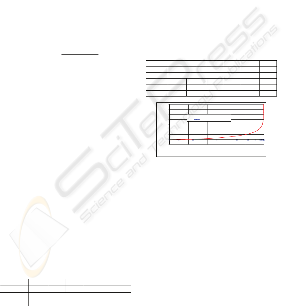
Figure 1 shows the graphical presentation of the
solution of the equations (Girdzijauskas S.,
Moskaliova V., 2005, p. 26).
Table 3.
Kp
100000 10 4 2 1.4
K/Kp
0.00001 0.1 0.25 0.5 0.71
LIRR
0.1632 0.18 0.20 0.25 0.33
Kp
1.2 1.1 1.05 1.03 1.01 1
K/Kp
0.83 0.91 0.95 0.97 0.99 1.00
LIRR
0.41 0.50 0.61 0.70 0.91 2.49
0.0
0.2
0.4
0.6
0.8
1.0
1.2
1.4
1.6
00.20.40.60.81
Market filling degree
Investment rate of return
Logistic rate of return
Normal rat e of return
Source: worked out by the authors with the data from Table 2.
Figure 1: Graph of investment heat (or of the growth of
internal rate of return).
The economic stability is strongly influenced by
the financial bubbles. The classical definition of a
financial bubble was introduced by Ch. Kindleberger
in 1978. Figure 1 clearly demonstrates that when the
investment is approaching the limit, i. e., reaching
the K
p
value, the threat of the bubble formation
appears (Streimikiene D., Girdzijauskas S., 2009,
2008).
The bubble is an exponentially growing increase
in price of an asset or a set of assets in a continuous
process when the initial increase in price is
determined by the vanishing decrease of the capital
niche, and the following growth of the internal rate
of return. It creates false expectations for a further
continuous growth in profitability and hence attracts
the new members of the market – in most cases,
profiteers who are interested in the profit brought by
MODELING THE FRAGILE ECONOMIC SITUATIONS
169

the asset trade rather than in the assets' capacity to
generate income.
3 CONCLUSIONS
• The possibilities for the application of the
logistic models in solving the economic
problems provide the opportunity to study the
formation of the financial bubbles.
• The practical modeling of the economic
bubbles allows to understand the assumptions
for the formation of the fragile economic
situations. Experts in economics should
improve their qualification by developing new
competences in the market estimation.
• The explored example of the logistic or
limited model should help to work out the
effective means for the prediction of the
economic situations.
REFERENCES
Girdzijauskas S. A., Streimikiene D., Dubnikovas M.,
2009. Analysing Banking Capital with Loglet Lab
Software Package. Transformations in Business &
Economics, p. 45-56.
Girdzijauskas S., Streimikiene D., et al, 2009. Formation
of Economic Bubbles: Causes and Possible
Preventions. Technological and Economic
Development of Economy, p. 267-280.
Girdzijauskas S., Streimikiene D., 2009. Application of
Logistic Models for Stock Market Bubbles Analysis.
Journal of Business Economics and Management, p.
45.
Girdzijauskas S., 2006. Logistine kapitalo valdymo teorija
: determinuotieji metodai : monografija. Vilnius.
Girdzijauskas S., Moskaliova V., 2005. Instability
modelling of financial pyramids. 5th International
Scientific and Practical Conference on Environment,
Technology, Resources, Jun 16-18, Rezekne, Latvia,
p. 26-32.
Streimikiene D., Girdzijauskas S.A., 2008. Logistic
growth models for analysis of sustainable growth.
Transformations in business & economics, p. 218-235.
Streimikiene D., Girdzijauskas S., 2009. Assessment of
post-Kyoto climate change mitigation regimes impact
on sustainable development. Renewable & sustainable
energy reviews, p. 118-130.
Girdzijauskas S., Streimikiene D., 2008. Logistic growth
models for analysis of stocks markets bubbles. World
Congress on Engineering, Imperial Coll London.
Engineering and Computer Science, p. 1166-1170.
Girdzijauskas S., Pikturna A., Ivanauskas F., et al., 2008.
Investigation of the elasticity of the price bubble
functions. 20th International Conference/Euro Mini
Conference on Continuous Optimization and
Knowledge-Based Technologies (EurOPT 2008), May
20-23, Neringa, Lithuania, p. 131-136.
Girdzijauskas S., Cepinskis J., Jurkonyte E., 2008.
Transformations in Insurance Market: Modern
Accounting Method of Insurance Tariffs.
Transformations in Business & Economics, p. 143-
153.
Girdzijauskas S.A., 2008. The Logistic Theory of Capital
Management: Deterministic Methods – Introduction.
Transformations in Business & Economics, p. 22-163
Gronskas H.Y., Streimikiene D., Girdzijauskas S.A., 2008.
Economy, Anti-economy and Globalisation.
Transformations in Business & Economics, p. 166-
168.
Merkevicius E., Garsva G., Girdzijauskas S., et al., 2007.
Predicting of Changes of Companies' Financial
Standings on the Basis of Self-organizing Maps. 9th
International Conference on Enterprise Information
Systems (ICEIS 2007), Funchal, Portugal, p. 416-419.
Moskaliova V., Girdzijauskas S., 2006. The Risk of
Investment: Determinate Models. 7th International
Baltic Conference on Databases and Information
Systems, Vilnius, Lithuania, p. 91-100.
CSEDU 2010 - 2nd International Conference on Computer Supported Education
170
