
CONVEX SHAPE RETRIEVAL FROM EDGE MAPS BY THE USE OF
AN EVOLUTIONARY ALGORITHM
A. Nezhinsky, J. Kruisselbrink and F. Verbeek
Leiden University, LIACS, Niels Bohrweg 1, The Netherlands
Keywords:
Evolutionary algorithm, Model based segmentation, Shape retrieval.
Abstract:
There is a need for a high-throughput approach for extracting biological shapes from images. The approach
for automated extraction of convex biological shapes presented in this paper is an Evolutionary Algorithm. As
opposed to existing model based segmentation methods this approach is uniform for different images, needs
no training set and is initialized automatically. The process of finding the shape is considered an optimization
problem and for that reason an Evolutionary Algorithm was a good candidate for a solution. The results show
that the proposed Evolutionary Algorithm gives a fast solution for pattern recognition and shape extraction.
1 INTRODUCTION
Pattern recognition is crucial for the analysis of large
image datasets in bio–imaging and many success-
ful applications have been described in the litera-
ture. The first step in many applications is to seg-
ment a meaningful biological structure from images
and remove the background, despite its position, ro-
tation and scale. Images in biology are acquired un-
der different conditions which affects quality, bright-
ness, contrast, lighting conditions and the amount of
noise. Consequently, extraction as well as processing
of shapes from the images might be hampered. For
our analysis we want to find an uniform way to over-
come these problems.
Since many biological shapes (cell, embryo etc.) can
be approximated by a convex shape we will propose
a method for extraction of convex-shaped structures
from images. Our approach is not meant for recog-
nition and discrimination between certain predefined
shapes, but for the recognition and the extraction of
the most prominent convex shape within the image.
The Evolutionary Algorithm (EA) will extract the ob-
ject with its shape closest to a convex shape and with
the best edge gradient. In most cases this is the bio-
logical structure.
Though many model based segmentation techniques
(T.F.Cootes et al., 2009), (M.Kass et al., 1987),
(F.Leymarie and M.D.Levine, 1993), (Y.N.Wu et al.,
2007), (J.A.Sethian and A.James, 1999) are already
successfully used, we want to investigate the possi-
bilities of an EA being able to extract convex shapes
from images. Thereby we want to look at the advan-
tages of an EA over other approaches and evaluate the
difficulties.
Figure 1 shows the general image process flow in
which the proposed method and the preprocessing
step are incorporated for shape extraction. Edge maps
are used as input images, since edges can be used as
distinctive features for shapes. An EA is used to ex-
tract the convex shapes from these edge maps.
Input image
Edge Map
Shape fitting by EA
Resulting Image
Figure 1: Data flowchart.
The paper is organized as follows. In section 2 exist-
ing approaches are discussed. Section 3 gives a short
overview of our approach. Section 4 addresses the
proposed EA used for shape recognition. In sections 5
experimental results are shown and they are discussed
in section 6.
221
Nezhinsky A., Kruisselbrink J. and Verbeek F. (2010).
CONVEX SHAPE RETRIEVAL FROM EDGE MAPS BY THE USE OF AN EVOLUTIONARY ALGORITHM.
In Proceedings of the First International Conference on Bioinformatics, pages 221-225
DOI: 10.5220/0002742502210225
Copyright
c
SciTePress
2 EXISTING APPROACHES
Most widely used methods are: active shape mod-
els (ASM) (T.F.Cootes et al., 2009); (F.J.Verbeek
et al., 2004), active snakes (or contours) (M.Kass
et al., 1987) (F.Leymarie and M.D.Levine, 1993), de-
formable templates (Y.N.Wu et al., 2007) and level-
set based methods (LSM) (J.A.Sethian and A.James,
1999).
Most model based segmentation methods are con-
cerned with the retrieval of certain pre–defined shapes
from the images.
A classic ASM approach needs a large training set.
Instances not matching the training set may fail. In
our approach no training set is needed.
With the ASM, deformable templates and the active
snake approach the initialization of the shape model
must be located close to the shape we are looking for.
The LSM approach and some other approaches also
suffer from high computational complexity.
3 APPROACH OVERVIEW
We want to develop an approach which is very flexi-
ble. While existing approaches like active snakes are
very flexible models, we want an even more flexible
one, where the initialization shape does not need to
be set (besides that it is a convex shape) and no train-
ing set is needed. An approach that does not require
predefined shapes for initialization could be applied
to different kind of images without any significant pa-
rameter change.
3.1 Image Preprocessing
Edge location within each image is efficiently repre-
sented by the magnitude of the gradient, which will be
the basis for the shape retrieval. Therefore we trans-
form the input image into a gray scale or a binary
representation from which the edge map is computed.
Any state of the art edge detector can be used for this
purpose.
Thus for each (pixel) position in the image we
have: | ▽ f(x,y) | as the magnitude of the gradient
(R.Gonzales and R.Woods, 2001) on the edge map.
We normalize this value between 0 and 1 and will de-
note the normalized magnitude of gradient as g
′
. The
normalized edge map will be used as the input for our
algorithm.
3.2 Structure of Candidate Solutions
The convex shape C is represented as minimal set of
points making up the convex hull:
C = {(x
1
,y
1
),...,(x
n
,y
n
)} (1)
The points are represented by xy–coordinates of pix-
els in the edge map. n denotes the number of points
used to approximate the shape.
For C we aim to find a convex shape with the largest
edge strength (as high as possible g
′
) in the edge map,
cf Figure 2.
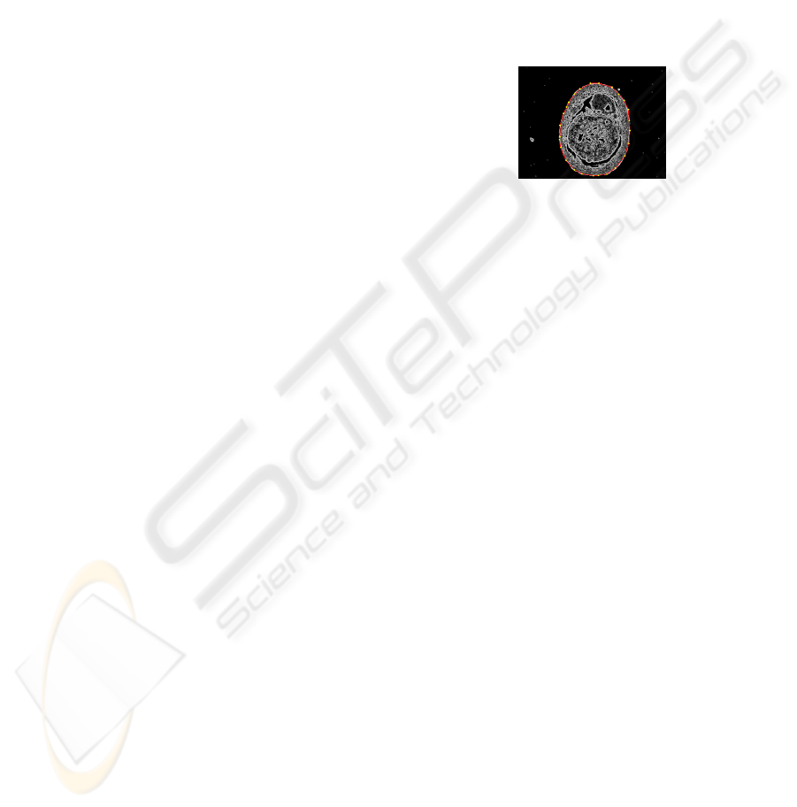
Figure 2: An example edge map of a light microscope im-
age of the embryo of Emys orbicularis. C is denoted as a
red contour. Yellow dots are the points making up C.
The process of finding C is considered an optimiza-
tion problem; given a large number of candidate so-
lutions (shapes) we are trying to find the optimal one.
For that reason an EA was a good candidate for a so-
lution.
When a solution (a contour) is found, the coordinates
of C are transferred to the initial image and the found
shape is cut out.
4 AN EA FOR CONVEX SHAPE
RECOGNITION
Evolutionary Algorithms (EA) (T.B¨ack, 1996) are
typically suitable for solving global optimization
problems (K.Deb, 2001), in particular when the solu-
tion space is very large and no straightforward analyt-
ical solution exists or can be found. In an EA, a popu-
lation of candidate solutions is evolved toward better
solutions by introducing computer analogues for re-
combination, mutation and selection.
The outline of a generic EA reads:
t = 0
Initialize P(t)
Evaluate P(t)
while not terminate do
P’(t) = SelectMates (P(t))
P’’(t) = Recombine (P’(t))
P’’’(t) = Mutate (P’’(t))
P(t + 1) = Select (P(t) \cup P’’’(t))
t = t + 1
end while
BIOINFORMATICS 2010 - International Conference on Bioinformatics
222

Here, t denotes the generation counter, P(t) =
{A
1
,.. .,A
µ
} is the population
1
of µ candidate solu-
tions (or individuals), and the functions SelectMates,
Recombine, Mutate, and Select represent the differ-
ent genetic operators. At the end of each iteration the
fitness Φ(A(t + 1)) of each individual in the new pop-
ulation is generated and the individuals of P(t+1) are
sorted by their fitness.
For the application of the principles of evolutionary
computation to the problem at hand one needs a suit-
able representation for the candidate solutions and a
method to determine the quality of the candidate so-
lutions which can serve as a fitness function for the
optimization.
4.1 Individual Representation
An individual A is represented by a collection of
points (cf.3.2). Each point has a value which is the
normalized gradient g
′
(x,y) (cf.3.1). An individual
can be represented as a finite set of points on a planar
space:
A = {(x
1
,y
1
),.. .,(x
n
,y
n
)} (2)
The convex hull shape is determined by the boundary
points of a point collection. We will denote this col-
lection of convex boundary points C
j
for individual
A
j
. The subset of points in A
j
construct the convex
shape C
j
for individual j as shown in Figure 3. Thus
C
j
⊇ A
j
.
Figure 3: a) The representation of an individual A
j
as a col-
lection of points, b) an individual A
j
and its convex hull C
j
,
c) convex boundary points C
j
.
4.2 Genetic Operators
For this specific application we only use mutation.
For each individual the following applies: every point
in the individual is mutated with a probability p
mut
.
The general rule for the approximation of p
mut
is the
formula p
mut
= 1/l, where l is the length of a bit string
of properties of an individual; in our case the num-
ber of points of A. When mutation is applied to a
point (x,y) its coordinates are mutated within some
(small) mutation area O
mut
around the old position of
1
We use notation P, not for probability, but for the pop-
ulation in an EA as is done in (T.B¨ack, 1996).
the point. A mutation fails if the mutated pixel is out-
side the image of if g
′
(x,y) = 0 (there is no gradient
at all). Then O
mut
is enlarged enabling a more global
mutation.
4.3 Utility Function
The quality (or fitness) of a candidate solution is com-
posed by the following:
1. i
C
is the fraction of all points of A which are
present on convex hull C:
i
C
=
|C|
|A|
→ max (3)
2. ¯g is the average gradient value of all points of A:
¯g =
∑
i=n
i=1
g
′
(x
i
,y
i
)
n
→ max (4)
3. b
C
is the normalized average gradient value of
points of the convex hull C (of individual A). We
calculate the average gradient value of the image
between these points. We perform a 8-connected
Bresenham-style walk (J.D.Foley et al., 1990) be-
tween all subsequent points in C. Let the func-
tion B((x
i
,y
i
),(x
j
,y
j
)) denote the average gradi-
ent value taken over the euclidean distance be-
tween consecutive points (x
i
,y
i
) and (x
j
,y
j
):
b
C
=
∑
i=i
C
−1
i=0
B((x
i
,y
i
),(x
j
,y
j
))
i
C
→ max (5)
4. σ
C
is the standard deviation of the convex hull
border segment length, normalized by the use of
average side distance. Let d((x
i
,y
i
),(x
j
,y
j
)) de-
note the euclidean distance between consecutive
points (x
i
,y
i
) and (x
j
,y
j
), d
avg
is the average dis-
tance of all these points.
σ
C
= e
(−1.0/d
avg
)·
s
∑
i=i
C
−1
i=0
d((x
i
,y
i
),(x
i+1
,y
i+1
))−d
avg
i
C
→ max (6)
Since parameters (i
C
, ¯g,b
C
,σ
C
) need be optimized si-
multaneously we are looking at a multi-objective op-
timization problem. The objectives can be conflict-
ing, for example, increase of the points on convex
hull can lead to lower gradient values. In our ap-
proach we aggregate the multiple objective functions
into an univariate problem by making use of the con-
cept of Desirability Functions (DF) and Desirability
Index (DI) (D.Steuer, 1999). We also make use of a
simple DF where for each parameter i we make use of
a power function f(i) = i
a
(all parameters are in a nor-
malized representation, it remains in the interval [0,1]
for any exponent a. To combine the DF’s into one
overall quality value we use a aggregation of all the
parameters. The following product fitness function is
parametrized as follows:
Φ(~a
j
(t)) = i
C
a
0
· ¯g
a
1
· b
C
a
2
· σ
C
a
3
→ max (7)
CONVEX SHAPE RETRIEVAL FROM EDGE MAPS BY THE USE OF AN EVOLUTIONARY ALGORITHM
223
4.4 Implementation
The number of points m in each individual can be set
depending on the precision of the prediction we want
to retrieve. Obviously a lower m gives less accurate
shape, while a higher m gives a more precise shape
but is computationaly more expensive.
The individuals are initialized with:
x
a
j
= U(0,ImageX), j = (1,.. .,n)
y
a
j
= U(0,ImageY), j = (1, ...,n) (8)
The convex shape C is calculated using the Graham
scan (R.L.Graham, 1972) algorithm with a time com-
plexity of O(m) (m is the number of points). Since the
algorithm needs a sorted list the points are sorted on
the x-coordinate by insertion sort.
Parent selection is repeated for each individual in the
new population (µ times). For the selection, tourna-
ment size q = 5 is chosen as one of the common set-
tings. A larger q results in less selective pressure. No
crossover is used, as it did not yield better results. As
a mutation rate of 1/m is most commonly used in EA,
the mutation rate for this implementation is chosen
accordingly, hence p
mut
= 1/m.
By means of empirical testing we found the following
settings fit for our problem: a
0
= a
1
= 1, a
2
= 2, a
3
=
0.5.
5 EXPERIMENTS AND RESULTS
For all tests we use a standard gradient operator – the
Sobel (R.Gonzales and R.Woods, 2001) edge detector
for the edge map creation.
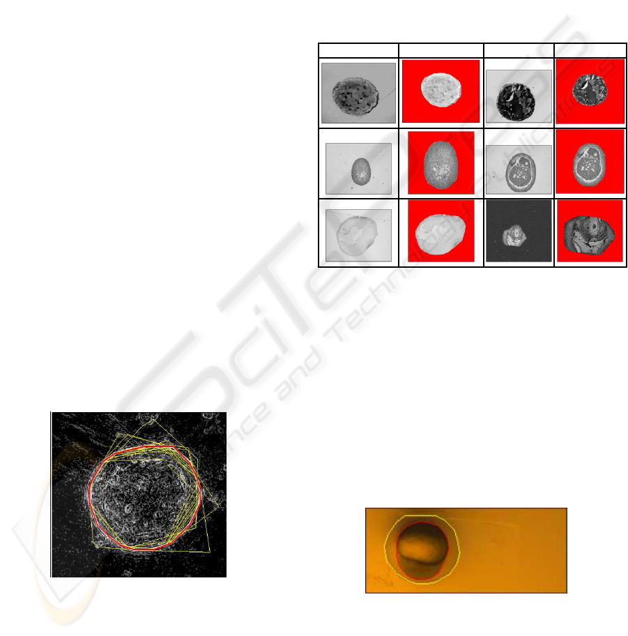
Figure 4: Snapshot of algorithm in search of best solution.
The process of finding the best solution is shown in
Figure 4. Thin yellow lines represent candidate solu-
tions. The bright red line represents the best solution
(with highest Φ).
5.1 Results: Finding a Convex Hull
Images from various fields in biology, containing con-
vex shapes were used for this test. The results are
shown in Table 1. As can be seen the shapes that
might be of interest are accurately retrieved. On
aIntel(R) Pentium(R) 4 CPU 3.2GHz this took on av-
erage 3 seconds.
Table 1: Some results of our algorithm applied to images
from different fields in biology after running for 70 genera-
tions and 2800 function–evaluations.
Input output input output
5.2 Results: Finding a Convex Hull
within a Convex Hull
In this section we will show that it is also possible to
retrieve a convex shape from another convex shape.
We have used and tested the approach for our par-
ticular data - images of zebrafish in the early de-
velopment. The images were acquired using Leica
MZ16FA light microscope in 24-bit color at a resolu-
tion of 2592 × 1944 pixels. Time–lapse acquisition is
accomplished in automated fashion over time T(5 –
10h).
Figure 5: Zebrafish embryo in early stage.
As can be seen in Figure 5 the shape of zebrafish
embryos in early stages can be described as a de-
formed circle being the embryo (red shape in Figure
5), encapsulated in a larger (deformed) circle being
the membrane (yellow shape in Figure 5).
BIOINFORMATICS 2010 - International Conference on Bioinformatics
224
In our case to extract the embryo shape from the im-
age we run the convexhull extraction algorithm twice.
First are looking for the outer convex shape. The mo-
ment the approximation of the outer shape (the mem-
brane) is complexed we try to find the inner shape
(the embryo), which is then the convexshape with the
largest edge strength within the membrane shape.
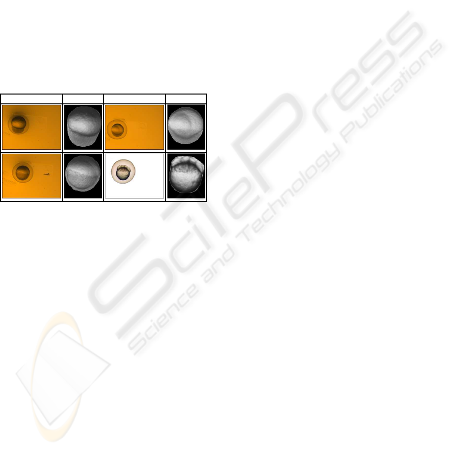
We have run the algorithm on a set of 600 images of
the zebrafish embryo. A few results shown in Table
2. As can be seen the embryo shapes were retrieved
accurately. The algorithm failed in cases where the
edge map was very weak (out of focus), which was
2% of our test set. On an Intel(R) Pentium(R) 4 CPU
3.2GHz this took up to 10 seconds.
Table 2: Some results of our algorithm applied to images
of zebrafish embryos after running for 300 generations and
24000 function–evaluations.
Input output Input images
6 DISCUSSION AND
CONCLUSION
In this paper, we have described the use of the EA for
the recognition of convex shaped objects and tested it
for different biological images.
We have demonstrated the application of the EA ap-
proach to different images and the possibility to re-
trieve both single convex shape (cf 5.1) as the possi-
bility to retrieve a convex shape from another convex
shape (cf 5.2).
In our approach the shape is not predefined like in
most models based segmentation methods, but can be
any convex shape within an image (assuming there
is one convex shape in the image, we are looking
for). Also, our approach does not need a training
set like ASM does and can be used without signif-
icant changes for different applications within bio–
imaging.
The results are promising and our future direction is
to apply this strategy in high-throughput applications
for screening and compare it against other methods.
This form of fast automated image analysis is indis-
pensable for such approaches.
ACKNOWLEDGEMENTS
This work was supported by the Smartmix program of
the Netherlands Ministry of Economic Affairs. Spe-
cial thanks to G. Lamers for assistance with image
acquisition and L. Bertens for providing images.
REFERENCES
D.Steuer (1999). Multi-criteria-optimization and desirabil-
ity indices. Technical Report 20/99, University of
Dortmund, Statistics Department,.
F.J.Verbeek, D.D.Rodrigues, H.Spaink, and A.Siebes
(2004). Data submission of 3d image sets to a bio-
molecular database using active shape models and a
3d reference model for projection. Proceedings SPIE
/5304/, Internet Imaging V. 13-23.
F.Leymarie and M.D.Levine (1993). Tracking deformable
objects in the plane using an active contour model.
IEEE Transactions on Pattern Analysis and Machine
Intelligence. Vol. 15, No. 6.
J.A.Sethian and A.James (1999). Level set methods and fast
marching methods : Evolving interfaces in compu-
tational geometry, fluid mechanics, computer vision,
and materials science. Cambridge University Press.
J.D.Foley, Dam, A., S.K.Feiner, and J.F.Hughes (1990).
Computer Graphics: Principles and Practice.
Addison-Wesley.
K.Deb (2001). Multi-Objective Optimization using Evolu-
tionary Algorithms. Wiley Interscience Series in sys-
tems and Optimization.
M.Kass, A.Witkin, and D.Terzopoulos (1987). Snakes: Ac-
tive contour models. International Journal of Com-
puter Vision. Vol. 1, No. 4.
R.Gonzales and R.Woods (2001). Digital Image Process-
ing. Addison-Wesley, London, 2nd edition.
R.L.Graham (1972). An efficient algorithm for determining
the convex hull of a finite. Information Processing
Letters 1.
T.B¨ack (1996). Evolutionary Algorithms in Theory and
Practice: Evolution Strategies, Evolutionary Pro-
gramming, Genetic Algorithms. Oxford Univ. press.
T.F.Cootes, C.J.Taylor, D.H.Cooper, and J.Graham (2009).
Active shape models - their training and application.
Computer Vision and Image Understanding, Vol. 61,
No. 1.
Y.N.Wu, Z.Si, C.Fleming, and Zhu, S. (2007). Deformable
template. IEEE International Conference on Com-
puter Vision.
CONVEX SHAPE RETRIEVAL FROM EDGE MAPS BY THE USE OF AN EVOLUTIONARY ALGORITHM
225
