
ENTR
OPIC ANALYSIS AND SYNTHESIS OF BIOSIGNAL
COMPLEXITY
Tuan D. Pham
School of Engineering and Information Technology, University of New South Wales, Canberra, ACT 2600, Australia
Keywords:
Entropy, Complexity, Geostatistics, Information Fusion, Mass Spectrometry Data.
Abstract:
Analysis of complexity of biological time-series data is investigated to gain knowledge about the biosignal
predictability. Using modern biological data such as mass spectral, this complexity information can be uti-
lized to identify novel biomarkers for drug discovery, early disease detection and therapeutic treatment. To
enhance the complexity analysis, a probabilistic fusion scheme, which is an alternative to the assumption of
the independence of probabilistic models, is applied to synthesize the information given by different entropy
methods.
1 INTRODUCTION
The notion of complexity can be defined as a scien-
tific study of systems which change irregularly over
time or space (Havel, 1995). Thus, understanding
the behaviors of dynamical systems in terms of pre-
dictability is a key purpose of the study of complexity.
There are several new perspectives developed on the
study of complexity in the physical and natural sci-
ences over last few decades. Theories such as nonlin-
ear dynamic systems, self-organization, catastrophe,
self-organized criticality, antichaos, and chaos appear
to offer novel perspectives on the long-standing prob-
lems of developing scientific measures of informa-
tion in the specific domain from which they emerge.
Depending on a particular discipline, these methods
for studying complexity have been characterized as
constituting everything from a major paradigm shift
which challenges established scientific beliefs to the
refinement of current methodology (Sprott, 2003).
An entropy-based measure of systems complex-
ity known as approximate entropy (ApEn) (Pincus,
1991) and its extended family - sample entropy (Sam-
pEn) (Richman and Moorman, 2000) and multiscale
entropy (MSE) (Costa et al, 2002) have been recently
proposed to quantify the complexity of physiologi-
cal and biological data. A low value of the approx-
imate entropy indicates the time series is determinis-
tic (low complexity); whereas a high value indicates
the data is subject to randomness (high complexity)
and therefore difficult to predict. In other words,
lower entropy values indicate more regular time se-
ries; whereas higher entropy values indicate more ir-
regular time series. Both ApEn and SampEn esti-
mate the probability that the sequences in a dataset
which are initially closely related remain closely re-
lated, within a given tolerance, on the next incremen-
tal comparison. ApEn differs from SampEn in that
its calculation involves counting a self-match for each
sequence of a pattern, which leads to bias in ApEn
(Pincus and Goldberger, 1994). SampEn is precisely
the negative natural logarithm of the conditional prob-
ability that two sequences similar for m points remain
similar at the next point, where self-matches are not
included in calculating the probability. Thus a lower
value of SampEn also indicates more self-similarity
in the time series. In addition to eliminating self-
matches, the SampEn algorithm is simpler than the
ApEn algorithm, requiring approximately one-half as
much time to calculate. SampEn is largely indepen-
dent of record length and displays relative consistency
under circumstances where ApEn does not (Richman
and Moorman, 2000).
It has been pointed that ApEn suffers from two
major drawbacks (Lewis and Short, 2007): (1) be-
cause it is a function of the length of the sequence
under study, it yields entropy values lower than ex-
pected for short sequences because its calculation in-
volves counting a self-match for each sequence and
this leads to bias (Pincus and Goldberger, 1994) ; (2)
it can be inconsistent with different testing conditions
using different parameters of the entropy index. Sam-
115
D. Pham T. (2010).
ENTROPIC ANALYSIS AND SYNTHESIS OF BIOSIGNAL COMPLEXITY.
In Proceedings of the Third International Conference on Bio-inspired Systems and Signal Processing, pages 115-120
DOI: 10.5220/0002326501150120
Copyright
c
SciTePress

pEn does not count self-matches and therefore can re-
duce bias. It has been found that SampEn can pro-
vide better relative consistency than ApEn because
it is largely independent of sequence length (Rich-
man and Moorman, 2000). MSE measures complex-
ity of time series data by taking into account multi-
ple time scales, and uses SampEn to quantify the reg-
ularity of the data. All of these three methods de-
pend on the selection of the two parameters known
as m and r: parameter m is used to determine the se-
quence length, whereas parameter r is the tolerance
threshold for computing pattern similarity. Results
are sensitive to the selections of these two parameters
and it has recently been reported that good estimates
of these parameters for different types of signals are
not easy to obtain (Lu et al, 2008). In this paper we
introduce a new entropy method called GeoEntropy
(GeoEn) which can provide an analytical procedure
for estimating the conrtol parameter r. We then apply
various entropy methods to study the complexity or
predictability of cancer using mass spectrometry data,
which are complex and large datasets. To improve
the entropy analysis, we use a novel probabilistic fu-
sion framework based on the engineering hypothesis
of permanence of ratio to combine the results from
different entropy algorithms.
1.1 GeoEntropy
Let z(X) be a regionalized variable which has charac-
teristics in a given region D of a spatial or time contin-
uum (Matheron, 1989). In the setting of a probabilis-
tic model, a regionalized variable z(X) is considered
to be a realization of a random function Z(X). In such
a setting, the data values are samples from a particular
realization z(X) of Z(X). We now consider n observa-
tion: z(X
α
), α = 1,... , I; taken at locations or times α.
If the objects are points in time or space, the possibil-
ity of infinite observations of the same kind of data is
introduced by relaxing the index α. The regionalized
variable is therefore defined as z(X) for all X ∈ D ,
and {z(X
α
),α = 1,..., I} is viewed as a collection of
a few values of the regionalized variable.
We now consider that each measured value in the
dataset has a geometrical or time point in the respec-
tive domain D , which is called a regionalized value.
The family of random variables {Z(X ),X ∈ D}, is
called the random function. The variability of a re-
gionalized variable z(X) at different scales can be
measured by calculating the dissimilarity between
pairs of data values, denoted by z(X
α
) and z(X
β
), lo-
cated at geometrical or time points α and β in a spa-
tial or time domain D, respectively (from now on
we address point/domain to imply either geometri-
cal or time point/domain). The measure of this semi-
dissimilarity, denoted by γ
αβ
, is computed by taking
half of the squared difference between the pairs of
sample values (the term semi is used to indicate the
half difference) as
γ
αβ
=
1
2
(X
α
− X
β
)
2
(1)
The two points x
α
and x
β
in space or time can be
linked by a space or time lag h = X
α
− X
β
(we use h
here as a scalar but its generalized form is a vector
to indicate various spatial orientations). Now let the
semi-dissimilarity depend on the lag h of the point
pair, we have
γ
α
(h) =
1
2
[(z(X
α
+ h) − z(X
α
)]
2
(2)
Using all samples pairs in a dataset, a plot of
the γ(h) against the separation h is called the semi-
variogram. The function γ(h) is referred to as the
semi-variance and defined as
γ(h) =
1
2N(h)
∑
(α,β)|h
αβ
=h
[z(X
α
) − z(X
β
)]
2
(3)
where N(h) is the number of pairs of data points
whose locations are separated by lag h.
The semi-variance defined in (3) is known as the
experimental semi-variance and its plot against h is
called the experimental semi-variogram, to distin-
guish it from the theoretical semi-variogram that char-
acterizes the underlying population. The theoretical
semi-variogram is thought of a smooth function repre-
sented by a model equation; whereas the experimental
semi-variogram estimates its form. The behavior of
the semi-variogram can be graphically illustrated by
the theoretical semi-variogram using the spherical or
the Matheron model which is defined as (Isaaks and
Srivastava, 1989)
γ(h) =
(
s
h
1.5
h
g
− 0.5(
h
g
)
3
i
: h ≤ g
s : h > g
(4)
where g and s are called the range and the sill of the
theoretical semi-variogram, respectively.
The concept of regionalized variables and its mod-
eling of variability in space continuum by means of
the semi-variogram have been described. What can
be observed is that the range g of the semi-variogram
presents an idea for capturing the auto-relationship
of the time-series data: within the range g, the data
points are related; when h > g, information about
relationship between the data points becomes satu-
rated and not useful. Based on this principle of the
BIOSIGNALS 2010 - International Conference on Bio-inspired Systems and Signal Processing
116

semi-variogram, the length of the sub-sequences of
the time-series data X can be appropriately chosen
to be the range g, which ensures an optimal study of
self-similarity of the signal, that is m = g(X). To ad-
dress the criterion of similarity/dissimilarity between
the sub-sequences, we can establish its lower bound
as the absolute difference between two consecutive
interval of the semi-variance or the absolute one-step
semi-variance difference: r = |γ(h) − γ(h + 1)|, or
multi-step semi-variance difference: r = |γ(h)−γ(h +
c)| where c is a positive constant. Having defined
the subsequence length m and the similarity criterion
r, determination of GeoEn can be obtained using the
principle of either ApEn or SampEn.
GeoEn algorithm for calculating the complexity of
time-series data is outlined as follows (Pham, 2009).
1. Compute the semi-variance of X
N
and its range
g(X
N
)
2. Set vector length m = g(X
N
)
3. Construct vectors of length m, X
1
to X
N−m
, de-
fined as
X
i
= (x
i
,x
i+1
,.. . ,x
i+m−1
), 1 ≤ i ≤ N − m
4. Set semi-variance lag h = 1, . ..,min
i
[g(X
i
)]
5. Compute distance between X
i
and X
j
as
d(X
i
,X
j
) = |γ
X
i
(h) − γ
X
j
(h)| (5)
6. Set the criterion of similarity r as follows.
r = |γ
X
i
(h) − γ
X
i
(h + 1)| (6)
7. Calculate either ApEn or SampEn for each h to
obtain multiscale GeoEn(X
N
,h).
2 PROBABILISTIC FUSION
Based on the engineering paradigm of the perma-
nence of updating ratios, which asserts that the rates
or ratios of increments are more stable than the incre-
ments themselves, as an alternative to the assumption
of the full or conditional independence of probabilis-
tic models; Journel introduced a scheme for informa-
tion fusion of diverse sources (Journel, 2002). This
scheme allows the combination of data events without
having to assume their independence. This informa-
tion fusion is described as follows.
Let P(A) be the prior probability of the occurence
of data event A; P(A|B) and P(A|C) be the probabil-
ities of occurence of event A given the knowledge
of events B and C, respectively; P(B|A) and P(C|A)
the probabilities of observing events B and C given
A, respectively. Using Bayes’ law, the posterior
probability of A given B and C is
P(A|B,C) =
P(A,B,C)
P(B,C)
=
P(A)P(B|A)P(C|A,B)
P(B,C)
(7)
The simplest way for computing the two proba-
bilistic models is to assume the model independence,
giving
P(C|A,B) = P(C|A) (8)
and
P(B,C) = P(B)P(C) (9)
Thus, (7) can be rewritten as
P(A|B,C)
P(A)
=
P(A|B)
P(A)
P(A|C)
P(A)
(10)
However, the assumption of conditional indepen-
dence between the data events usually does not statis-
tically perform well and leads to inconsistencies in
many real applications (Journel, 2002). Therefore,
an alternative to the hypothesis of conventional data
event independence should be considered. The per-
manence of ratios based approach allows data events
B and C to be incrementally conditionally dependent
and its fusion scheme gives
P(A|B,C) =
1
1 + x
=
a
a + bc
∈ [0,1] (11)
where
a =
1 − P(A)
P(A)
, b =
1 − P(A|B)
P(A|B)
,
c =
1 − P(A|C)
P(A|C
, x =
1 − P(A|B,C)
P(A|B,C)
.
An interpretation of the fusion expressed in (11) is
as follows. Let A is the target event which is to be up-
dated by events B and C. The term a is considered as
a measure of prior uncertainty about the target event
A or a distance to the occurrence of A without any up-
dated evidence. The term x is the distance to the target
event A occurring after observing evidences given by
both events B and C. The ratio c/a is then the incre-
mental (increasing or decreasing) information of C to
that distance starting from the prior distance a. Simi-
larly, the ration x/b is the incremental information of
C starting from the distance b. Thus, the permanence
of ratios provides the following relation
x
b
≈
c
a
(12)
which says that the incremental information about C
to the knowledge of A is the same after or before
ENTROPIC ANALYSIS AND SYNTHESIS OF BIOSIGNAL COMPLEXITY
117
0 2000 4000 6000 8000 10000 12000
0
100
200
300
400
500
600
700
m/z
Intensity
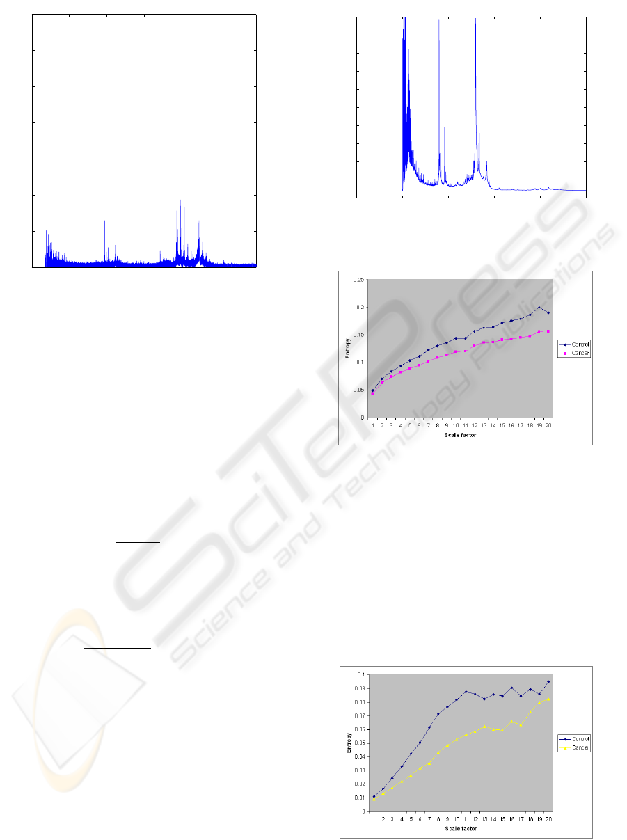
Figure 1: Ovarian mass spectrometry data: disease sample.
knowing B. In other words, the incremental contri-
bution of information from C about A is independent
of B. This expression relaxes the restriction of the as-
sumption of full independence of B and C.
For the generation of k data events E
j
, j = 1, . ..,k;
the conditional probability provided by a succession
of (k − 1) permanence of ratios is given as
P(A|E
j
, j = 1,..., k) =
1
1 + x
∈ [0,1] (13)
where
x =
∏
k
j=1
d
j
a
k−1
≥ 0
a =
1 − P(A)
P(A)
d
j
=
1 − P(A|E
j
)
P(A|E
j
)
, j = 1,..., k
It is clear that expression (13) requires only the
knowledge of the prior probability P(A), and the k
elementary single conditional probabilities P(A|E
j
),
j = 1,..., k, which can be independently computed.
3 EXPERIMENTAL ANALYSIS
AND SYNTHESIS OF
BIOSIGNAL COMPLEXITY
We used a public MS-based ovarian cancer dataset,
the ovarian high-resolution SELDI-TOF, to carry out
−5000 0 5000 10000 15000 20000
0
10
20
30
40
50
60
70
80
90
100
m/z
Intensity
Figure 2: Ovarian mass spectrometry data: control sample.
Figure 3: Mean entropy values of cancer and control groups
using MSE.
the entropic analysis and synthesis. The dataset was
obtained from the FDA-NCI Clinical Proteomics Pro-
gram Databank. The ovarian cancer data consist of
100 control samples and 170 cancer samples. The
length of each sample is 15,154 m/z values. Figures
1 and 2 show the plots of typical ovarian, and control
samples, respectively.
Mass spectrometry (MS) in proteomics has been
used to study the regulation, timing, and location of
Figure 4: Mean entropy values of cancer and control groups
using MSE with m values of GeoEn.
BIOSIGNALS 2010 - International Conference on Bio-inspired Systems and Signal Processing
118
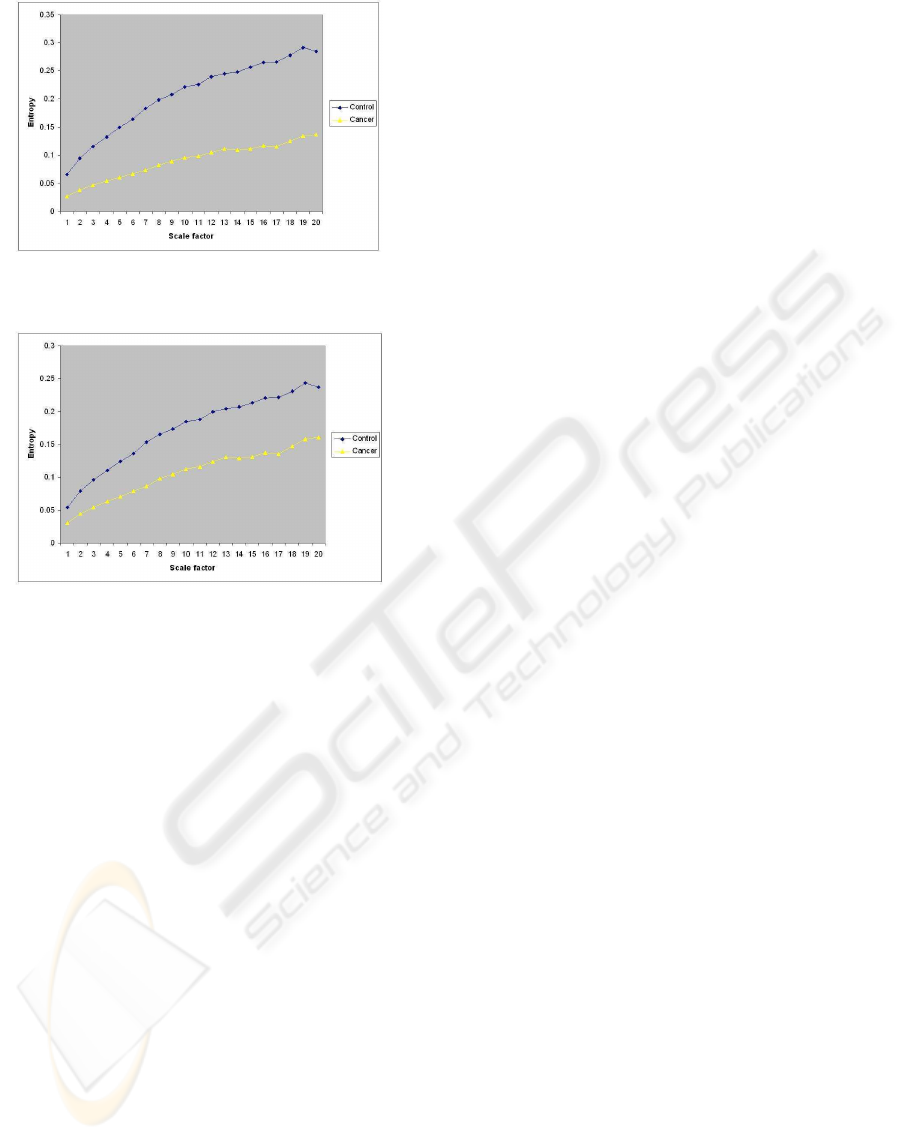
Figure 5: Probabilistic combination of entropy values of
cancer and control groups.
Figure 6: Average combination of entropy values of cancer
and control groups.
protein expression. Interaction studies seek to under-
stand how protein pair between themselves and other
cellular components interact to constitute to more
complex models of the molecular machines. In par-
ticular, protein expression profiles or expression pro-
teomics can be used for large-scale protein charac-
terization or differential expression analysis that has
many applications such as disease classification and
prediction, new drug treatment and development, vir-
ulence factors, and polymorphisms for genetic map-
ping, and species determinants (Adam et al, 2001).
In comparison with transcriptional profiling in func-
tional genomics, proteomics has some obvious advan-
tages in that it provides a more direct approach to
studying cellular functions because most gene func-
tions are characterized by proteins. Current study on
MS data concerns with peak detection for biomarker
discovery and pattern classification for disease predic-
tion. In this study, we examined the complexity of this
type of MS data and applied the proposed classifica-
tion scheme to classifying cancer and control samples
and compared the performance of the proposed meth-
ods with other methods.
Applying the experimental semi-variogram, we
obtained the range about 20 for both cancer and con-
trol populations and set this value to be the value m
for the entropy calculation. For the entropy estimates
using MSE, the constant values of m and r are 2 and
0.15, respectively. Figure 3 shows the plots of the
mean entropy values of the cancer and control groups
using MSE. Some difference of MSE values between
the cancer and control groups can be observed; how-
ever, the entropy values of the two groups increase
with increasing scales. Figures 4 shows the plots of
the mean entropy values of the cancer and control
groups using MSE procedure with the values of m ob-
tained from GeoEn approach. The entropy profiles
of the cancer and control populations obtained from
MSE-based GeoEn can distinguish the complexities
between the groups. The entropy values of the con-
trol group take higher values than those of the cancer.
Both cancer and control populations tend to increase
with increasing values of h.
To enhance the complexity analysis, we applied
the permanence-of-ratio fusion to combine the two
updating results obtained from MSE and GeoEn given
the prior results estimated from SampEn. In this fu-
sion, P(A) is the prior probability of the complexity of
the data given by SampEn, P(A|B) and P(A|B) are the
probabilities of the complexity obtained from MSE
and GeoEn, respectively, given the knowledge pro-
vided by SampEn. These three defined probabilities
are ready to calculate the three parameters a, b and c
to estimate the updated probability P(A|B,C) defined
in (11). Figure 5 shows the fused entropy values. It
can be observed that the separation of the complexity
profiles becomes better in comparisons with the pro-
files produced separately by MSE and GeoEn. Fig-
ure 6 shows the entropy profiles taken as the average
of the two results given by MSE and GeoEn. It can
be seen that combination by averaging does not yield
better results than the probabilistic fusion scheme.
4 CONCLUSIONS
Approximate entropy was introduced for the analysis
of short time series. Sample entropy was developed
as a modified version of ApEn to offer the advantage
of some independence on time series length. More
recently, multiscale entropy has been introduced by
averaging time series data with different intervals or
scales which are then analyzed by sample entropy.
All of these three entropy-based algorithms rely on
the heuristic estimates of m and r. The GeoEn ap-
proach offers an analytical procedure for the estima-
tion of these parameters. Data fusion has been widely
used for improving results from multiple sources of
information. This study has combined advantages
of entropy-based methods by means of a data fusion
ENTROPIC ANALYSIS AND SYNTHESIS OF BIOSIGNAL COMPLEXITY
119

method. Furthermore, what we have reported is the
application of a most recently developed data combi-
nation scheme which does not impose the strong in-
dependent assumption of probabilistic models. The
approaches studied herein can be applied to many
types of biosignals for early disease prediction and
biomarker discovery where the entropy profiles can
be used as novel features in pattern classification pro-
cess.
ACKNOWLEDGEMENTS
This work was supported by UNSW@ADFA Rec-
tor Start-up Grant and Australian Research Council’s
Discovery Projects funding scheme (project number
DP0877414).
apalike)
REFERENCES
Adam BL, Vlahou A, Semmes OJ, Wright Jr GL. Pro-
teomic approaches to biomarker discovery in prostate
and bladder cancers, Proteomics 2001, 1: 1264-1270.
Costa M, Goldberger AL, Peng CK. Multiscale entropy
analysis of complex physiologic time series. Phys.
Rev. Lett. 2002, 89: 068102-1 - 068102-4.
Costa M, Goldberger AL, Peng CK, Multiscale entropy
analysis of biological signals. Physical Review E
2005, 71: 021906-1-021906-18.
Havel I. Scale Dimensions in Nature. Int. J. General Sys-
tems 1995, 23: 303-332.
Isaaks EH, Srivastava RM. An Introduction to Applied Geo-
statistics. New York: Oxford University Press; 1989.
Journel AG. Combining knowledge from diverse sources:
An alternative to traditional data independence hy-
potheses. Mathematical Geology 2002, 34: 573-595.
Lewis MJ, Short AL. Sample entropy of electrocardio-
graphic RR and QT time-series data during rest and
exercise. Physiological Measurement 2007, 28: 731-
744.
Lu S, Chen X, Kanters JK, Solomon IC, Chon KH. Auto-
matic selection of the threshold value r for approx-
imate entropy, IEEE Trans. Biomedical Engineering
2008, 55: 1966-1972.
Matheron G. Estimating and Choosing. Berlin: Springer-
Verlag; 1989.
Pham TD. GeoEntropy: a measure of complexity
and similarity, Pattern Recognition 2009, DOI:
10.1016/j.patcog.2009.08.015), in-print.
Pincus SM. Approximate entropy as a measure of sys-
tem complexity. Proc. Natl. Acad. Sci. U.S.A. 1991,
88:2297-2301.
Pincus SM, Goldberger AL. Physiological time-series anal-
ysis: what does regularity quantify? Am. J. Physiol.
1994, 4: H1643-1656.
Richman JS, Moorman JR. Physiological time-series anal-
ysis using approximate entropy and sample en-
tropy. Amer. J. Physiol. Heart Circ. Physiol. 2000,
278:H2039-H2049.
Sprott JL. Chaos and Time-Series Analysis. New York: Ox-
ford; 2003.
BIOSIGNALS 2010 - International Conference on Bio-inspired Systems and Signal Processing
120
