
FUZZY TOPOGRAPHIC MODELING IN WIRELESS SIGNAL
TRACKING ANALYSIS
Eddie C. L. Chan, George Baciu and S. C. Mak
The Hong Kong Polytechnic University, Hung Hom, Kowloon, Hong Kong
Keywords: Wireless signal tracking, Topographic Mapping, Received Signal Strength, Fuzzy Logic.
Abstract: Fuzzy logic modelling can be applied to evaluate the behaviour of Wireless Local Area Networks (WLAN)
received signal strength (RSS). The behavior study of WLAN signal strength is a pivotal part of WLAN
tracking analysis. Previous analytical model has not been addressed effectively for analyzing how the
WLAN infrastructure affected the accuracy of tracking. In this paper, we propose a novel fuzzy spatio-
temporal topographic model. We implemented the proposed model with a large (9.34 hectare), built-up
university, over 2,000 access points to survey and collect WLAN received signal strength (RSS). We
applied the Nelder-Mead (NM) method to simplify our previous work on fuzzy color map into a
topographic (line-based) map. The new model can provide a detail and quantitative strong representation of
WLAN RSS. Finally, it serves as a quicker reference and efficient analysis tool for improving the design of
WLAN infrastructure.
1 INTRODUCTION
Wireless Local Area Networks (WLAN) tracking
analysis is a crucial part for deploying the efficient
indoor positioning system. The analytical models
can be used to visualize the distribution of signal and
help to improve the design of positioning systems,
for example by eliminating installation of WLAN
access points (APs) and shortening the sampling
time of WLAN received signal strength (RSS) in
location estimation. The most typical techniques for
locating WLAN enabled device are location-
fingerprinting-based (LF-based). LF based method
(Taheri et al., 2004)(J. Kwon et al., 2004)(K.
Kaemarungsi and P. Krishnamurthy, 2004)(B. Li et
al., 2005) locate a device by accessing a training
database containing the location fingerprint to
estimate the location. Location fingerprint (LF) is a
set of the RSSs and coordinates in a region.
Recent research on WLAN RSS analytical
model (K. Kaemarungsi and P. Krishnamurthy, 2004)
and (N. Swangmuang and P. Krishnamurthy, 2008)
are based on the accuracy of positioning systems and
proximity graphs, such as Voronoi diagram,
clustering graph. They assume the distribution of the
RSS is in Gaussian and pair wise. Some research
works (N. Swangmuang and P. Krishnamurthy,
2008), (M. B. Kjaergaard and C. V. Munk, 2008),
and (S. Fang et al., 2008) ignores the radio signal
properties. Such assumptions may ignore or distort
the real behavior of RSS and provides inadequate
and inaccurate RSS analysis. The fuzzy visualization
map concepts widely applied in other fields, such as
temperature, rainfall and atmosphere. Topographic
mapping has been also highly recognized as a
comprehensive method to visualize geographical
information, such as the reflectance of slope and
terrain. NM method also is used in many other fields
such as data mining (S. Satapathy et al., 2007) and
antenna optimization (B. Kolundzija and D. Olcan,
2003). Fuzzy, topographic and NM modelling could
well be applied to modelling in WLAN RSS
analytical model.
In this paper, we propose a novel analytical
model that provides a visualization of the RSS
distribution. We make use of the Nelder-Mead (NM)
method to simplify our pervious works on the multi-
layer fuzzy color model (C. L. Chan et al., 2008) to
topographic (line-based) model. We develop a
topographic model as analytical tools for evaluating
and visualizing where the RSS is denser and
clustering different RSS in different topographic
level. The proposed model offers two benefits. First,
it serves as a quicker reference and efficient analysis
tool. Second, it can provide a detail and quantitative
strong representation of WLAN RSS.
17
Chan E., Baciu G. and Mak S. (2009).
FUZZY TOPOGRAPHIC MODELING IN WIRELESS SIGNAL TRACKING ANALYSIS.
In Proceedings of the International Joint Conference on Computational Intelligence, pages 17-24
DOI: 10.5220/0002312700170024
Copyright
c
SciTePress

The rest of this paper is organized as follows:
Section 2 presents the topographic model design.
Section 3 presents the experimental setup of large
scale site RSS surveying in 9.34 hectare campus area
over 2,000 access points. Section 4 discusses the
analysis result of obstacles, human bodies and
WLAN APs location. Finally, Sections 5 offers our
conclusion and future work.
2 TOPOGRAPHIC MODEL
DESIGN
The basic idea of topographic model is to plot a
curve connecting minimum points where the
function has a same particular RSS value. The sets
of APs are known as topographic line nodes.
Topographic line nodes are the APs residing on the
topographic lines around contour region. In this
section, we introduce the major operations of
topographic model including propagation-based
algorithm, fuzzy membership function in our
previous work (C. L. Chan et al., 2008), topographic
line node measurement, Nelder-Mead method and
topographic model generation.
2.1 Propagation-based Algorithm
The propagation-based algorithm (K. Kaemarungsi
and P. Krishnamurthy, 2004) which is used to
calculate the RSS as follows:
wallLossddrdr
kikii
−−= )(log10)()(
,1000,
α
(1)
where
{
}
n
in
dddD ℜ∈= |...
1
is a set of
locations, R =
{
}
n
in
rrr ℜ∈|...
1
is a set of sampling
LF vector respect to known d
i
, α is the path loss
exponent (clutter density factor) and wallLoss is the
sum of the losses introduced by each wall on the line
segment drawn at Euclidean distance d
i,k
.
2.2 Fuzzy Membership Function
In this subsection, our fuzzy membership function
has been published in (C. L. Chan et al., 2008) and
we will make use of it. Nonetheless, for
completeness in the following we briefly describe.
Using fuzzy logic, the proposed model offers an
enhanced LF hyperbolic solution that maps the RSS
from a 0 to 1 fuzzy membership function. Instead of
using a numeric value, the fuzzy logic determines
the RSS as “strong”, “normal” and “weak”.
Figure 1: The RSS fuzzy membership graph.
The normalization distribution is used to represent
the fuzzy membership functions.
2
2
2
)(
2
1
)(
σ
μα
πσ
−
= exP
where p(x) is the probability function, x is the
normalized RSS, σ is the standard deviation of
normalized signal normalized strength in a region, μ
is the mean of signal strength in a region. The
WLAN network is fully covered for the whole
campus.
The membership function of term set,
μ(RSSDensity) = {Red, Green,Blue}. Red means the
signal strength density is high, green means the
signal strength is medium and blue means the signal
strength density is low. The fuzzy set interval of
blue is [0, 0.5], [0, 1] is green and [0.5, 1] is red.
For the blue region, σ = 0.5, μ = 0.
()
2
2
2
00.5
2
x
Blue
x
e
μ
π
−
<< =
(2)
For the green region, we substitute, σ = 0.5, μ = 0.5.
()
()
2
1
2
2
2
01
2
x
Green
xe
μ
π
−−
<< =
(3)
For the red region, σ = 0.5, μ = 1.
()
()
2
21
Re
2
0.5 1
2
x
d
xe
μ
π
−−
<< =
(4)
Figure 1shows the fuzzy membership function. X-
axis represents the normalized signal strength from 0
to 1 (from -93dBm to -15dBm). The width of
membership function depends on the standard
deviation of the RSS. The overlap area will be
indicated by mixed colors. We can use different
colored regions to represent the WLAN RSS
distribution. Conceptually we define a spatio-
temporal region as follows:
Assume that B is a finite set of RSS vector
belonging to a particular color region,
IJCCI 2009 - International Joint Conference on Computational Intelligence
18

where
{}
1
... |
n
ni
Bbbb=∈ℜ, i.e.,
i
bS∈ , SR
∀
∈ ,
and
[
]
,Slu∀∈ , where l is the lower bound of fuzzy
interval and u is a upper bound of fuzzy interval. To
analyze the distribution surfaces S, there always
exists a spatio-temporal mapping,
SBq →:
.
∫
=
S
dSSbxhxq )()()(
(5)
where h(x) is the characteristic function of S, i.e.,
⎩
⎨
⎧
=
0
1
)(xh
x
S
∈
,
x
S
∉
(6a)
(6b)
and b(S) is a weight function that specifies a prior on
the distribution of surfaces S. We can explicitly
define b(S) by (1). By (2), (3), (4), (5) and (6), the
RSS distribution can be illustrated.
2.3 Topographic Node
Each topographic node consists of three components
and can be expressed as < l, d, g >, in which l
represents topographic level, d represents the
locations of WLAN received signal, g represents the
gradient direction of the RSS distribution. The
spatial data value distribution mapped into the (x, y, l)
space, where the co-ordinate (x, y) represents the
location and l = f(x, y) describes a function mapping
from (x, y) co-ordinates to level l. The gradient
vector g denotes the direction of RSS where to
degrade in the space. The gradient vector can be
calculated by:
()
T
y
f
x
f
yxfg
⎟
⎟
⎠
⎞
⎜
⎜
⎝
⎛
Δ
Δ
Δ
Δ
=−= ,,
'
(7)
2.4 Nelder-Mead Method
The Nelder-Mead (NM) method is a commonly used
nonlinear optimization algorithm for finding a local
minimum of a function of several variables has been
devised by Nelder and Mead (J. Mathews and K.
Fink, 1998). It is a numerical method for minimizing
an objective function in a many-dimensional space.
Instead of using (1) and (2), we estimate the location
by NM method.
First, we collect the location fingerprint, r with an
unknown location (x,y). We define f(n)=|n-r|, where n
is any location fingerprint. Second, we select three
location fingerprints (LFs) to be three vertices of a
triangle.
We initialize a triangle BGW and function f is to
be minimized. Vertices B, G, and W, where f(B) is
the smallest value (best vertex), f(G) is the medium
value (good vertex), and f(W) is a largest value
(worst vertex). There are 4 cases when using NM
method. They are reflection, expansion, contraction
and shrink. We recursively use NM method until
finding the point which is the local minimum (nearest)
in B, G, W that they are the same value.
The midpoint of the good side is
2
B
G
M
+
=
(8)
2.4.1 Reflection using the Point R
The function decreases as we move along the side of
the triangle from W to B, and it decreases as we move
along the side from W to G. Hence it is feasible that
function f takes on smaller values at points that lie
away from W on the opposite side of the line
between B and G. We choose a test point R that is
obtained by “reflecting” the triangle through the side
BG. To determine R, we first find the midpoint M of
the side BG. Then draw the line segment from W to
M and call its length d. This last segment is extended
a distance d through M to locate the point R (See
Figure 2). The vector formula for R is
()2
R
MMW MW
=
+−= −
(9)
2.4.2 Expansion using the Point E
If the function value at R is smaller than the function
value at W, then we have moved in the correct
direction toward the minimum. Perhaps the minimum
is just a bit farther than the point R. So we extend the
line segment through M and R to the point E. This
forms an expanded triangle BGE. The point E is
found by moving an additional distance d along the
line joining M and R (See Figure 3). If the function
value at E is less than the function value at R, then
we have found a better vertex than R. The vector
formula for E is
()2
E
RRM RM
=
+− = −
(10)
2.4.3 Contraction using the Point C
If the function values at R and W are the same,
another point must be tested. Perhaps the function is
smaller at M, but we cannot replace W with M
FUZZY TOPOGRAPHIC MODELING IN WIRELESS SIGNAL TRACKING ANALYSIS
19

because we must have a triangle. Consider the two
midpoints C
1
and C
2
of the line segments WM and
MR, respectively (see Figure 4). The point with the
smaller function value is called C, and the new
triangle is BGC. Note. The choice between C
1
and C
2
might seem inappropriate for the two-dimensional
case, but it is important in higher dimensions.
C
1
= (M - W)/2 (11)
C
2
= R - (M - W)/2
(12)
2.4.4 Shrink toward B
If the function value at C is not less than the value at
W, the points G and W must be shrunk toward B (see
Figure 5). The point G is replaced with M, and W is
replaced with S, which is the midpoint of the line
segment joining B with W.
S = (B - W)/2 (13)
Figure 2: Reflection using
the Point R.
Figure 3: Expansion using the
Point E.
Figure 4: Constraction
using the Point C.
Figure 5: Shrink toward B.
2.5 Topographic Model Generation
We generate topographic model based on our
previous work (C. L. Chan et al., 2008) and NM
algorithm. We apply NM method to a many-
dimensional RSS distribution space problem to
simplify the fuzzy color map down to a contour
(line-based) map.
First, we select three LFs to be three vertices of a
triangle:
→
B
,
→
G
, and
→
W
, where
→
B
is a location with
high RSS (best vertex),
→
G
is a location with medium
RSS (good vertex), and
→
W
is a location with the low
RSS (worst vertex). The location vector of RSS at
x
k
,y
k
use in function, N(x, y). We use (1) to define
N(x, y). There are 4 cases when using NM method.
They are reflection, expansion, contraction and
shrink. We recursively use NM method until finding
the point which is the local minimum in
→
B
,
→
G
, and
→
W
that they are the same value. Table 1 summarizes
the procedure.
Table 1: Nelder-Mead Method Procedure.
IF f(R)<f(G), THEN Perform Case (i) {either reflect or
extend}
ELSE Perform Case (ii) {either contract or shrink}
BEGIN {Case(i).}
IF f(B)<f(R) THEN
replace W with R
ELSE
compute E and f(E)
IF f(E)<f(B) THEN
replace W with E
ELSE
replace W with R
ENDIF
ENDIF
END {Case (i)}
BEGIN {Case(ii).}
IF f(R)<f(W) THEN
replace W with R
ENDIF
compute C = (W + M)/2
or C = (M + R)/2 and f (C)
IF f(C)<f(W) THEN
replace W with C
ELSE
compute S and f(S)
replace W with S
replace G with M
ENDIF
END {Case (ii)}
A contour function is then used to plot a curve
connecting minimum points where the function has a
same particular value. We normalize the minimum
value between 0 and 1, and the contour line is 0.1 in
each level.
3 EXPERIMENTAL SETUP
In this section, we describe experiment setup in 9.34
hectare campus area. We use the same setting as
used in (J. Kwon et al., 2004), (R. Jan and Y. Lee,
2003), (Taheri et al., 2004), (K. Kaemarungsi and P.
Krishnamurthy, 2004), (K. Kaemarungsi and P.
Krishnamurthy, 2004), (W. Wong et al., 2005) and
(P. Bahl et al., 2000). RSS site survey measurement
will be in The Hong Kong Polytechnic University
(PolyU) campus. The approximate total area of the
campus is 9.34 hectare. A standard laptop computer
equipped with an Intel WLAN card and client
manager software was used to measure samples of
RSS from access points (APs) of PolyU campus.
IJCCI 2009 - International Joint Conference on Computational Intelligence
20
The WLAN card is chipset inside the laptop.
There are basically 26 buildings from Core A to
Core Z and 7 extra buildings with WLAN access.
Each core building is covered by at least 13 APs.
The radio frequency (RF) channels of IEEE 802.11b
are in the 2.4 GHz band which is shared by other
equipment in the industrial, scientific, and medical
(ISM) band such as Bluetooth. The number of non-
overlapping channels for 802.11b is three. We
observe that the RSS value reported by the WLAN
card is an average value over a sampling period and
in integral steps of 1 dBm. The received signal
sensitivity of the WLAN card also limits the range
of the RSS to be between -93 dBm and -15 dBm.
Nevertheless, the highest typical value of the RSS is
approximately -30 dBm at one meter from any AP.
The sampling schedule is to collect the RSS data
every 5 seconds. The vector of RSS data at each
location forms the location fingerprint with around
20 RSS elements in the vector. Total 27 locations of
measurement are chosen in the campus.
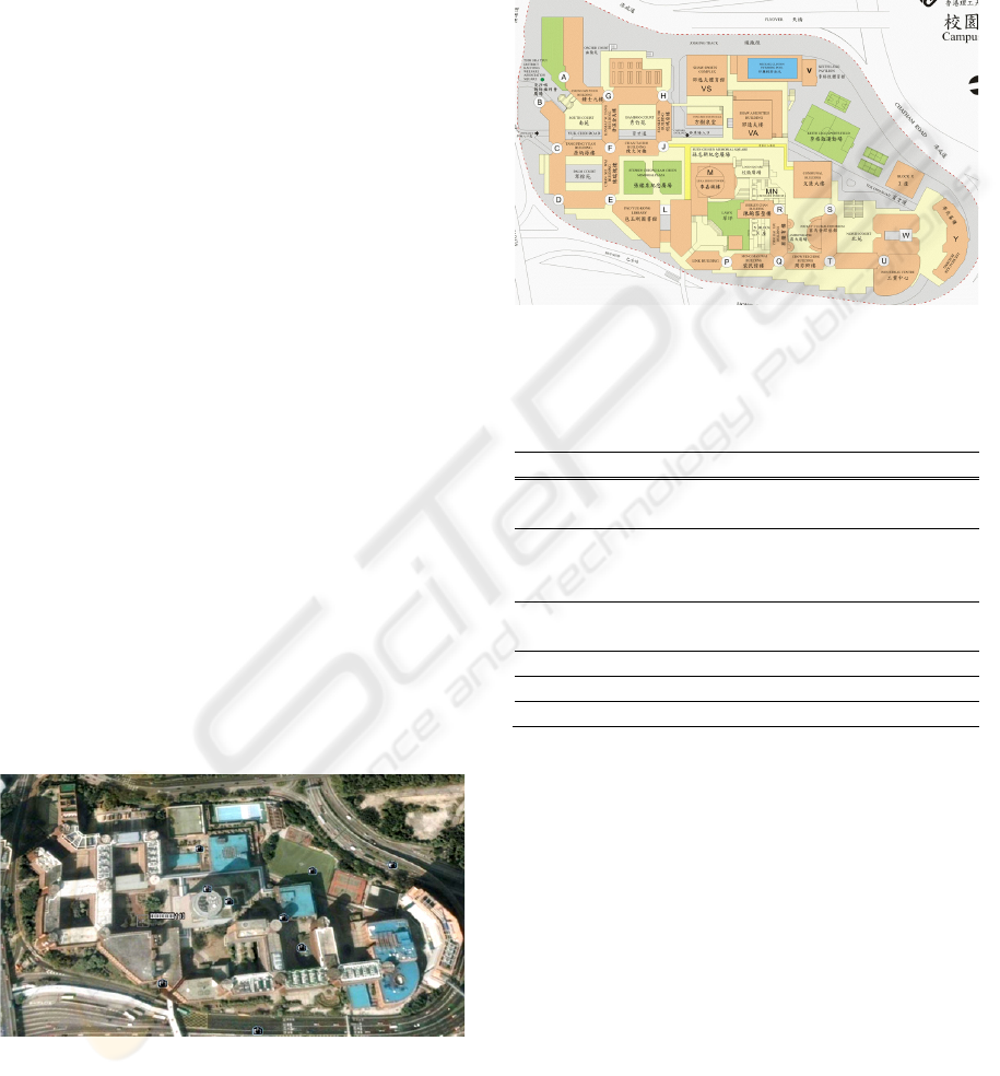
Figure 6 and 7 show the 27 locations site plan.
The radio channels used for each AP are channel 1,
6, and 11 respectively. The sampling will be taken
with two periods of time, (7:30am-9:30am (leisure)
and 4:30pm - 6:30pm (busy)). From (K.
Kaemarungsi and P. Krishnamurthy, 2004), the
presence or absence of people in the building
significantly affects the RSS values. The data were
collected four times with four different directions,
North, South, East and West. The duration of
sampling was 2 weeks with total 12 days (from Mon
to Sat). In mean while, temperature, weather,
sampling time and humidity were recorded. The
total number of RSS samples would be 12 days X 4
directions X 27 buildings X 20 APs X 2 times =
51840.
Figure 6: The satellite photo of PolyU campus from
Google Earth.
For 27 locations on the floor, we collected
environmental readings at these locations over two-
week period of time. At each testing location, we
picked a frequency 2.4GHz and calculated their
average amplitude respectively. Note that the RSS is
the received signal from a beacon packet, while the
spectrum energy is the ambient RF energy
corresponding to a specific frequency range. Table 2
summaries the campus area measurement setup
Figure 7: The site plan for PolyU Campus with 27
buildings.
Table 2: Summary of Experiment Setup in PolyU Campus.
Item Description
Total campus area 9.34 hectare
26 core + 7 extra buildings
Sampling period 2 weeks
7.30am - 9.30am
4.30pm - 6.30pm
RSS variation Between -93 dBm and -15
dBm
No. of sample points 51,840 sample points
WLAN channel 1, 6, and 11
Facing direction North, South, East, and West
4 DISCUSSION AND ANALYSIS
In this section, we discuss the effect of the presence
of human and LOS factor in our topographic model.
There are three RSS features to
be analyzed, LOS, the presence of human and RSS
variation.
4.1 Effect of LOS on RSS
Figure 8 and 9 show the effect of LOS in two major
clusters of RSS. The two major centers of high
intensity locate at F core and S core.
The distance between F core to S core buildings
is around 600m apart. The RSS should be covered
evenly. Moreover, between M core (Lee Ka Shing
FUZZY TOPOGRAPHIC MODELING IN WIRELESS SIGNAL TRACKING ANALYSIS
21
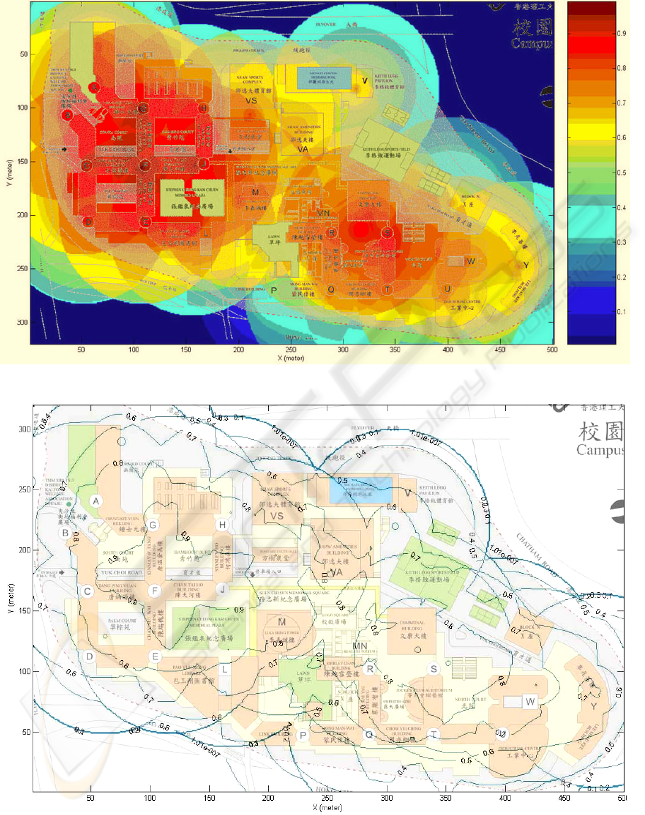
Figure 8: Fuzzy RSS Distribution with the campus floor plan.
Figure 9: Topographic RSS Distribution with the campus floor plan.
IJCCI 2009 - International Joint Conference on Computational Intelligence
22

Tower) to R core buildings (Shirley Chan Tower),
the RSS distribution is relatively low. The heights of
two buildings in M core and R core are around 80m
and 70m respectively. The distance between M to R
core is around 200m apart.
As we can see the topographic map in Figure 11a
and 11b, the slope of contour line from M core to R
core is steep in the edge area, it means that the RSS
is weaken quickly in the middle from M core to R
core due to NLOS effects. For LOS conditions, RSS
should fit into log-normal distribution. A multi-story
building in a campus area will experience lower
signal strengths within tall buildings due to the
absence of LOS propagation.
4.2 Behavior Study on the Human’s
Presence
As the previous section mention, we collected the
RSS data in 2 periods, one is in the morning leisure
period (7.30am-9.30am) and the other is in the busy
evening period (4:30pm - 6.30pm). We would like to
observe the difference between two periods. Figure
10 and 11 show the difference RSS pattern which
the RSS collect in the two different time slot. We
can see that there is significant change of the RSS
value. Figure 11a shows the topographic region in
0.9 level is larger than Figure 11b. We can observe
the slope on Figure 11b degrades larger than Figure
11a. As a result, it verifies the effect of the user’s
presence can affect the mean of the RSS value.
4.3 Effect of the RSS Variation on
Accuracy
The accuracy of the tracking system is highly
dependent on RSS variation. If the standard
deviation of the RSS increases, the accuracy of the
tracking system falls. To maintain high accuracy, the
suggested standard deviation of RSS should be
under 4dBm in this paper. (Elsewhere, a standard
deviation of 2.13dBm has been assumed. (Taheri et
al., 2004)) However, as the standard deviation
depends on the real environment, including the
density of human traffic, in some situations the
standard deviation will be large.
(a) In the leisure morning period (b) In the busy evening period
Figure 10: RSS Distribution in Fuzzy Analytical Model.
(a) In the leisure morning period (b) In the busy evening period
Figure 11: RSS Distribution in Topographic Model.
FUZZY TOPOGRAPHIC MODELING IN WIRELESS SIGNAL TRACKING ANALYSIS
23

5 CONCLUSIONS
In this paper, we propose NM optimized topographic
model for RSS distribution. The new model provides
quicker references and efficient analysis tool for
improving the design of WLAN infrastructure to
achieve localization accuracy. In our university site
experiment, we provide a spatial analytical model
for WLAN tracking in a campus. The fuzzy
topographic RSS analytical map provides easier
understanding of WLAN RSS pattern in a region.
The usage of model can improve the efficiency
usage of WLAN infrastructure substantially. Future
work will consist in building a 3D pervasive
tracking and a dynamic spatio-temporal filtering
technique.
REFERENCES
Taheri, A. Singh, and A. Emmanuel, 2004. Location
fingerprinting on infrastructure 802.11 WLAN local
area networks (WLANs) using Locus. Proceedings of
the 29
th
Annual IEEE International Conference on
Local Computer Networks, pages 676–683.
J. Kwon, B. Dundar, and P. Varaiya, 2004. Hybrid
algorithm for indoor positioning using WLAN LAN.
Vehicular Technology Conference, 2004. VTC2004-
Fall.
K. Kaemarungsi and P. Krishnamurthy, 2004. Modeling of
indoor positioning systems based on location
fingerprinting. INFOCOM 2004. Twenty-third
AnnualJoint Conference of the IEEE Computer and
Communications Societies, 2, 2004.
B. Li, Y.Wang, H. Lee, A. Dempster, and C. Rizos, 2005.
Method for yielding a database of location fingerprints
in WLAN. Communications, IEE Proceedings-,
152(5):580–586, 2005.
N. Swangmuang and P. Krishnamurthy, 2008. Location
Fingerprint Analyses Toward Efficient Indoor
Positioning. Sixth Annual IEEE International
Conference on Pervasive Computing and
Communications, 2008, pages 101–109, 2008.
M. B. Kjaergaard and C. V. Munk, 2008. Hyperbolic
Location Fingerprinting- A Calibration-Free Solution
for Handling Differences in Signal Strength. Sixth
Annual IEEE International Conference on Pervasive
Computing and Communications, 2008, pages 110–
116, 2008.
S. Fang, T. Lin, and P. Lin, 2008. Location Fingerprinting
In A Decorrelated Space. Knowledge and Data
Engineering, IEEE Transactions on, 20(5):685–691,
2008.
S. Satapathy, J. Murthy, P. Reddy, V. Katari, S. Malireddi,
and V. Kollisetty, 2007. An Efficient Hybrid
Algorithm for Data Clustering Using Improved
Genetic Algorithm and Nelder Mead Simplex Search.
Conference on Computational Intelligence and
Multimedia Applications, 2007. International
Conference on, 1, 2007.
B. Kolundzija and D. Olcan, 2003. Antenna optimization
using combination of random and Nelder-Mead
simplex algorithms. Antennas and Propagation Society
International Symposium, 2003. IEEE, 1, 2003.
C. L. Chan, G. Baciu, and S. C. Mak, 2008. WLAN
Tracking Analysis in Location Fingerprint. to appear
in the IEEE WLAN and Mobile Computing,
Networking and Communications, 2008.
K. Kaemarungsi and P. Krishnamurthy, 2004. Properties
of indoor received signal strength for WLAN location
fingerprinting. Mobile and Ubiquitous Systems:
Networking and Services, 2004. MOBIQUITOUS
2004. The First Annual International Conference on,
pages 14–23, 2004.
R. Jan and Y. Lee, 2003. An indoor geolocation system for
WLAN LANs. Parallel Processing Workshops, 2003.
Proceedings. 2003 International Conference on, pages
29–34, 2003.
W. Wong, J. Ng, and W. Yeung, 2005. WLAN LAN
positioning with mobile devices in a library
environment. Distributed Computing Systems
Workshops, 2005. 25th IEEE International Conference
on, pages 633–636, 2005
P. Bahl, V. Padmanabhan, and A. Balachandran, 2000. A
Software System for Locating Mobile Users: Design,
Evaluation, and Lessons. online document, Microsoft
Research, February, 2000.
Taheri, A. Singh, and A. Emmanuel, 2004. Location
fingerprinting on infrastructure 802.11 WLAN local
area networks (WLANs) using Locus. Proceedings of
the 29th Annual IEEE International Conference on
Local Computer Networks, pages 676-683, 2004.
J. Mathews and K. Fink, 1998. Numerical Methods Using
MATLAB. Simon & Schuster, 1998.
IJCCI 2009 - International Joint Conference on Computational Intelligence
24
