CLUSTER ENSEMBLE SELECTION

Using Average Cluster Consistency

F. Jorge F. Duarte, Jo

ao M. M. Duarte, M. F

atima C. Rodrigues

GECAD - Knowledge Engineering and Decision Support Group, Instituto Superior de Engenharia do Porto, Porto, Portugal

Ana L. N. Fred

Instituto de Telecomunicac¸

oes, Instituto Superior T

ecnico, Lisboa, Portugal

Keywords:

Cluster ensemble selection, Cluster ensembles, Data clustering, Unsupervised learning.

Abstract:

In order to combine multiple data partitions into a more robust data partition, several approaches to produce

the cluster ensemble and various consensus functions have been proposed. This range of possibilities in the

multiple data partitions combination raises a new problem: which of the existing approaches, to produce the

cluster ensembles’ data partitions and to combine these partitions, best ﬁts a given data set. In this paper, we

address the cluster ensemble selection problem. We proposed a new measure to select the best consensus data

partition, among a variety of consensus partitions, based on a notion of average cluster consistency between

each data partition that belongs to the cluster ensemble and a given consensus partition. We compared the

proposed measure with other measures for cluster ensemble selection, using 9 different data sets, and the

experimental results shown that the consensus partitions selected by our approach usually were of better quality

in comparison with the consensus partitions selected by other measures used in our experiments.

1 INTRODUCTION

Data clustering goal consists of partitioning a data set

into clusters, based on a concept of similarity between

data, so that, similar data patterns are grouped to-

gether and unlike patterns are separated into different

clusters. Several clustering algorithms have been pro-

posed in the literature but none can discover all kinds

of cluster structures and shapes.

In order to improve data clustering robustness and

quality (Fred, 2001), reuse clustering solutions (Strehl

and Ghosh, 2003) and cluster data in a distributed

way, various cluster ensemble approaches have been

proposed based on the idea of combining multiple

data clustering results into a more robust and better

quality consensus partition. The principal proposals

to solve the cluster ensemble problem are based on:

co-associations between pairs of patterns (Fred and

Jain, 2005; Duarte et al., 2006), mapping the cluster

ensemble into graph (Fern and Brodley, 2004), hyper-

graph (Strehl and Ghosh, 2003) or mixture model

(Topchy et al., 2004b) formulations, and searching for

a median partition that summarizes the cluster ensem-

ble (Jouve and Nicoloyannis, 2003).

A cluster ensemble can be built by using different

clustering algorithms (Duarte et al., 2006), using dis-

tinct parameters and/or initializations to the same al-

gorithm (Fred and Jain, 2005), sampling the original

data set (Topchy et al., 2004a) and using different fea-

ture sets to produce each individual partition (Topchy

et al., 2003).

One can also apply different consensus functions

to the same cluster ensemble. These variations in the

cluster ensemble problem leads to a question: “Which

cluster ensemble construction method and which con-

sensus function should one select for a given data

set?”. This paper addresses the implicit problem in

the previous question by selecting the best consensus

partition based on the concept of average cluster con-

sistency between the consensus partition and the re-

spective cluster ensemble.

The rest of this paper is organized as follows. In

section 2, the cluster ensemble problem formulation

(subsection 2.1), background work about cluster en-

semble selection (subsection 2.2) and the clustering

combination methods used in our experiments (sub-

section 2.3) are presented. Section 3 presents a new

approach for cluster ensemble selection, based on the

Jorge F. Duarte F., M. M. Duarte J., Fátima C. Rodrigues M. and L. N. Fred A. (2009).

CLUSTER ENSEMBLE SELECTION - Using Average Cluster Consistency.

In Proceedings of the International Conference on Knowledge Discovery and Information Retrieval, pages 85-95

DOI: 10.5220/0002308500850095

 SciTePress

notion of average cluster consistency. The experi-

mental setup used to assess the performance of our

proposal is described in section 4 and the respective

results are presented in section 5. Finally, the conclu-

sions appear in section 6.

2 BACKGROUND

2.1 Cluster Ensemble Formulation

Let X = {x

, ···, x

} be a set of n data patterns and let

P = {C

, ···,C

} be a partition of X into K clusters.

A cluster ensemble P is deﬁned as a set of N data

partitions P

of X :

P = {P

, ···, P

}, P

= {C

, ···,C

}, (1)

where C

is the k

cluster in data partition P

which contains K

clusters, and

∑

k=1

| = n,

∀l ∈ {1, · · · , N}.

There are two fundamental phases in combin-

ing multiple data partitions: the partition generation

mechanism and the consensus function, that is, the

method that combines the N data partitions in P . As

introduced before, there are several ways to generate

a cluster ensemble P , such as, producing partitions of

X using different clustering algorithms, changing pa-

rameters and/or initializations for the same clustering

algorithm, using different subsets of data features or

patterns, projecting X to subspaces and combinations

of these. A consensus function f maps a cluster en-

semble P into a consensus partition P

∗

, f : P → P

∗

such that P

∗

should be robust and consistent with P ,

i.e., the consensus partition should not change (signif-

icantly) when small variations are introduced in the

cluster ensemble and the consensus partition should

reveal the underlying structure of P .

2.2 Cluster Ensemble Selection

As previously referred, the combination of multiple

data partitions can be carried out in various ways,

which may lead to very different consensus partitions.

This diversity causes the problem of picking the best

consensus data partition from all the produced ones.

In (Hadjitodorov et al., 2006) work, a study was

conducted on the diversity of the cluster ensemble and

its relation to the consensus partition quality. Four

measures were deﬁned in order to assess the diver-

sity of a cluster ensemble, by comparing each data

partition P

∈ P with the ﬁnal data partition P

∗

. The

adjusted Rand index (Hubert and Arabie, 1985) was

used to assess the agreement between pairs of data

clusterings (Rand(P

, P

∗

) ∈ [0, 1]). Values close to 1

means that the clusterings are similar.

The ﬁrst measure, Div

∗

, P ), is deﬁned as the

average diversity between each clustering P

∈ P and

the consensus partition P

∗

. The diversity between P

and P

∗

is deﬁned as 1 − Rand(P

, P

∗

). Formally, the

average diversity between P

∗

and P is deﬁned as:

Div

∗

, P ) =

∑

l=1

1 −Rand(P

, P

∗

). (2)

Previous work (Kuncheva and Hadjitodorov, 2004)

showed that the cluster ensembles that exhibit higher

individual variation of diversity generally obtained

better consensus partitions.

The second measure, Div

∗

, P ), is based in this

idea and is deﬁned as the standard deviation of cluster

ensemble individual diversity:

Div

∗

, P ) =

N − 1

∑

l=1



1 − Rand



, P

∗



− Div



(3)

where Div

is Div

∗

, P ).

The third diversity measure, Div

∗

, P ) is based

on the intuition that the consensus partition, P

∗

, is

similar to the real structure of the data set. So, if the

clusterings P

∈ P are similar to P

∗

, i.e., 1 − Div

close to 1, P

∗

is expected to be a high quality con-

sensus partition. Nevertheless, as it is assumed that

cluster ensembles with high individual diversity vari-

ance are likely to produce good consensus partitions,

the third measure also includes a component associ-

ated to Div

∗

, P ). It is formally deﬁned as:

Div

∗

, P ) =

(1 −Div

+ Div

), (4)

where Div

corresponds to Div

∗

, P ).

The forth measure, Div

∗

, P ), simply consists

of a ratio between the standard deviation of the clus-

ter ensemble individual diversity and the average di-

versity between P

∗

and P , as shown in equation 5.

Div

∗

, P ) =

Div

∗

, P )

Div

∗

, P )

(5)

The four previously referred measures were com-

pared in (Hadjitodorov et al., 2006) and the au-

thors concluded that only Div

∗

, P ) and, specially,

Div

∗

, P ) measures shown some correlation with

the quality of the consensus partition. Despite that,

in some data sets the quality of the ﬁnal data parti-

tions increased as Div

∗

, P ) and Div

∗

, P ) also

increased, in several other data sets it did not oc-

curred. The authors recommended that one should

select the cluster ensembles with the median values

KDIR 2009 - International Conference on Knowledge Discovery and Information Retrieval

of Div

∗

, P ) or Div

∗

, P ) to choose a good con-

sensus partition.

In other work (Strehl and Ghosh, 2003), the best

consensus partition P

is thought as the consen-

sus partition P

∗

that maximizes the Normalized Mu-

tual Information (NMI) between each data partition

∈ P and P

∗

, i.e., P

= argmax

∗

∑

NMI(P

∗

, P

NMI(P

∗

, P

) is deﬁned as:

NMI(P

∗

, P

) =

MI(P

∗

, P

)

H(P

∗

)H(P

))

, (6)

where MI(P

∗

, P

) is the mutual information between

∗

and P

(eq. 7) and H(P) is the entropy of P (eq. 8).

The mutual information between two data partitions,

∗

and P

, is deﬁned as:

MI(P

∗

, P

) =

∗

∑

Prob(i, j)

Prob(i)Prob( j)

, (7)

with Prob(k) =

, where n

is the number of patterns

in the k

cluster of P, and Prob(i, j) =

∗

∩C

The entropy of a data partition P is given by:

H(P) = −

∑

k=1

Prob(k)log Prob(k). (8)

Therefore, the Average Normalized Mutual Infor-

mation (ANMI(P

∗

, P )) between the cluster ensemble

and a consensus partition, deﬁned in eq. 9, can be

used to select the best consensus partition. Higher

values of ANMI(P

∗

, P ) suggest better quality consen-

sus partitions.

ANMI(P

∗

, P ) =

∑

l=1

NMI(P

∗

, P

). (9)

2.3 WEACS

The Weighted Evidence Accumulation Clustering us-

ing Subsampling (WEACS) (Duarte et al., 2006) ap-

proach is an extension to Evidence Accumulation

Clustering (EAC) (Fred, 2001). EAC considers each

data partition P

∈ P as an independent evidence

of data organization. The underlying assumption of

EAC is that two patterns belonging to the same nat-

ural cluster will be frequently grouped together. A

vote is given to a pair of patterns every time they co-

occur in the same cluster. Pairwise votes are stored in

a n × n co-association matrix and are normalized by

the total number of combining data partitions:

co assoc

i j

∑

l=1

vote

i j

, (10)

where vote

i j

= 1 if x

and x

belong to the same clus-

ter C

in the data partition P

, otherwise vote

i j

= 0. In

order to produce the consensus partition, one can ap-

ply any clustering algorithm over the co-association

matrix co assoc.

WEACS extends EAC by weighting each pattern

pairwise vote based on the quality of each data par-

tition P

and by using subsampling in the construc-

tion of the cluster ensemble. The idea consists of per-

turbing the data set and assigning higher relevance to

better data partitions in order to produce better com-

bination results. To weight each vote

i j

in a weighted

co-association matrix, w co assoc, one or several in-

ternal clustering validity indices are used to measure

the quality of each data partition P

, and the corre-

sponding normalized index value, IV

, corresponds to

the weight factor. Note that the internal validity in-

dices assess the clustering results in terms of quan-

tities that involve only the features of the data set,

so no a priori information is provided. Formally,

w co assoc is deﬁned as

w co assoc

i j

∑

l=1

× vote

i j

, (11)

where S is a n×n matrix with S

i j

equal to the number

of data partitions where both x

and x

are simultane-

ously selected to belong to the same data subsample.

There are two versions of WEACS that corre-

spond to two different ways for computing the weight

factor IV

. The ﬁrst one, Single WEACS (SWEACS),

uses the result of only one clustering validity index to

assess the quality of P

, i.e., IV

= norm validity(P

where norm

validity(·) corresponds to a normalized

validity index function that returns a value in the

interval [0, 1]. Higher values correspond to bet-

ter data partitions. In the second version, Joint

WEACS (JWEACS), IV

is deﬁned as the average of

the output values of NumInd normalized validity in-

dex functions, norm validity

(·), applied to P

, i.e.,

∑

NumInd

m=1

norm validity

We used the following 10 internal clustering valid-

ity indices: Normalized Hubert Statistic (NormHub)

(Hubert and Schultz, 1975), Dunn index (Dunn,

1974), Davies-Bouldin index (DB) (Davies and

Bouldin, 1979), SD validity index (Halkidi et al.,

2001), the S Dbw validity index (Halkidi et al., 2001),

Caliski & Harabasz cluster validity index (Calin-

ski, 1974), Silhouette statistic (S) (Kaufman and

Roussesseeuw, 1990), index I (Maulik and Bandy-

opadhyay, 2002), XB cluster validity index (Xie and

Beni, 1991), and the Point-Symmetry index (PS)

(Chou et al., 2004).

NormHub and S indices are intrinsically normal-

ized in the interval [−1, 1] but only index values be-

tween 0 and 1 are considered to weight data pairwise

votes. In our experiments, for these two indices, we

CLUSTER ENSEMBLE SELECTION - Using Average Cluster Consistency

set all negative index values to 0. For some of the re-

maining indices, higher values implies better data par-

titions while for the others lower values corresponds

to the better data partitions. For this reason, for the

indices of the ﬁrst type, the normalized index value is

deﬁned as

norm

validity(P

) =

index(P

)

max

1≤m≤N

index(P

)

, (12)

where index(P

) is the index value for a partition in

the cluster ensemble P

∈ P and index(P

) is always

non-negative. For the indices of the second type, the

normalized index value is obtained by

norm validity(P

) =

min

1≤m≤N

index(P

)

index(P

)

. (13)

In the WEACS approach, one can use differ-

ent cluster ensemble construction methods, different

clustering algorithms to obtain the consensus par-

tition, and, particularly in the SWEACS version,

one can even use different cluster validity indices

to weight pattern pairwise votes. These constitute

variations of the approach, taking each of the pos-

sible modiﬁcations as a conﬁguration parameter of

the method. As shown in section 4, although the

WEACS leads in general to good results, no individ-

ual tested conﬁguration led consistently to the best re-

sult in all data sets. We used a complementary step to

the WEACS approach which consists of combining

all the ﬁnal data partitions obtained in the WEACS ap-

proach within a cluster ensemble construction method

using EAC. The interested reader is encouraged to

read (Duarte et al., 2006) for a detailed description

of WEACS.

3 AVERAGE CLUSTER

CONSISTENCY (ACC)

The idea behind Average Cluster Consistency (ACC)

measure is that if the similarity between the multiple

data partitions in the cluster ensemble and the consen-

sus partition is high, the quality of the consensus par-

tition will also be high. Some clustering combination

methods, such as the EAC and WEACS methods pre-

sented in subsection 2.3, usually produce better qual-

ity consensus data partitions when combining data

partitions with more clusters than the expected real

number of clusters K

. This difference in the number

of clusters usually leads to low similarity scores when

comparing two data partitions. For this reason, a new

concept for comparing data partitions was deﬁned. In

this new similarity measure between two data parti-

tions, P

and P

with K

>> K

, if each of the K

clusters C

∈ P

is a subset of a cluster C

∈ P

, i.e.

j C

,then the partitions P

and P

have the max-

imum degree of similarity. If the data patterns be-

longing to each cluster in P

are split into different

clusters in P

, the data partitions P

and P

are dis-

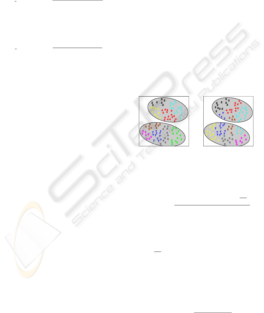
similar. Figure 1 shows an example of the previously

described situations. The ﬁgure includes two consen-

sus partitions (one in ﬁgure 1 (a) and another in ﬁg-

ure 1 (b)) each with K

= 2 clusters (shaded areas).

Inside each consensus partition’s clusters, there are

several patterns represented by numbers, which indi-

cate the cluster labels assigned to the data patterns in

a partition P

belonging to the cluster ensemble. Note

that the number of clusters of the partition P

is higher

than the number of clusters of the consensus partition

>> K

). On the left ﬁgure, a perfect similar-

ity between P

and P

is presented as all data patters

of each cluster C

belong to the same cluster in P

On the right ﬁgure, two dissimilar partitions are pre-

sented as the data patterns belonging to clusters 1, 5

and 7 in P

are divided in the two clusters of P

(a) similar partitions (b) dissimilar partitions

Figure 1: Example of Average Cluster Consistency motiva-

tion.

Our similarity measure between two partitions, P

∗

and P

, is then deﬁned as

sim(P

∗

, P

) =

∑

m=1

max

1≤k≤K

∗

|Inters

|(1 −

∗

)

(14)

where K

≥ K

∗

, |Inters

| is the cardinality of the

set of patterns common to the k

and m

clusters

of P

∗

and P

, respectively (Inters

= {x

∈ C

∗

∧

∈ C

). Note that in Eq. 14, |Inters

| is weighted

by (1 −

∗

) in order to prevent cases where P

∗

has

clusters with almost all data patterns and would ob-

tain a high value of similarity.

The Average Cluster Consistency measures the

average similarity between each data partition in the

cluster ensemble (P

∈ P ) and a target consensus par-

tition P

∗

, using the previously explained notion of

similarity. It is formally deﬁned by

ACC(P

∗

, P ) =

∑

i=1

sim(P

, P

∗

)

. (15)

KDIR 2009 - International Conference on Knowledge Discovery and Information Retrieval

From a set of possible choices, the best consensus par-

tition is the one that achieves the highest ACC(P

∗

, P )

value. Note that by the fact of using subsampling, the

ACC measure only uses the data patterns of the con-

sensus partition P

∗

that appear in the combining data

partition P

∈ P .

At the ﬁrst glance, this measure may seem to con-

tradict the observations by (Hadjitodorov et al., 2006)

and (Kuncheva and Hadjitodorov, 2004) which point

out that the clustering quality is improved with the in-

crease of diversity in the cluster ensemble. However,

imagine that each data partition belonging to a cluster

ensemble is obtained by random guess. The resulting

cluster ensemble is very diverse but does not provide

useful information about the structure of the data set,

so, it is expected to produce a low quality consensus

partition. For this reason, one should distinguish the

“good” diversity from the “bad” diversity. Our deﬁ-

nition of similarity between data partitions (Eq. 14)

considers that two apparently different data partitions

(for instance, partitions with different number of clus-

ters) may be similar if they have a common structure,

as shown in the ﬁgure 1 (a) example, and the outcome

is the selection of cluster ensembles with “good” di-

versity rather than the ones with “bad” diversity.

4 EXPERIMENTAL SETUP

We used 4 synthetic and 5 real data sets to assess the

quality of the cluster ensemble methods on a wide va-

riety of situations, such as data sets with different car-

dinality and dimensionality, arbitrary shaped clusters,

well separated and touching clusters and distinct clus-

ter densities. A brief description for each data set is

given below.

(a) Bars (b) Cigar (c) Spiral (d) Half Rings

Figure 2: Synthetic data sets.

Synthetic Data Sets. Fig. 2 presents the 2-

dimensional synthetic data sets used in our experi-

ments. Bars data set is composed by two clusters very

close together, each with 200 patterns, with increas-

ingly density from left to right. Cigar data set con-

sists of four clusters, two of them having 100 patterns

each and the other two groups 25 patterns each. Spiral

data set contains two spiral shaped clusters with 100

data patterns each. Half Rings data set is composed

by three clusters, two of them have 150 patterns and

the third one 200.

Real Data Sets. The 5 real data sets used in

our experiments are available at UCI repository

(http://mlearn.ics.uci.edu/MLRepository.html). The

ﬁrst one is Iris and consists of 50 patterns from each

of three species of Iris ﬂowers (setosa, virginica and

versicolor) characterized by four features. One of the

clusters is well separated from the other two overlap-

ping clusters. Breast Cancer data set is composed

of 683 data patterns characterized by nine features

and divided into two clusters: benign and malignant.

Yeast Cell data set consists of 384 patterns described

by 17 attributes, split into ﬁve clusters concerning ﬁve

phases of the cell cycle. There are two versions of

this dataset, the ﬁrst one is called Log Yeast and uses

the logarithm of the expression level and the other is

called Std Yeast and is a “standardized” version of

the same data set, with mean 0 and variance 1. Fi-

nally, Optdigits is a subset of Handwritten Digits data

set containing only the ﬁrst 100 objects of each digit,

from a total of 3823 data patterns characterized by 64

attributes.

In order to produce the cluster ensembles, we

applied the Single-Link (SL) (Sneath and Sokal,

1973), Average-Link (AL) (Sneath and Sokal, 1973),

Complete-Link (CL) (King, 1973), K-means (KM)

(Macqueen, 1967), CLARANS (CLR) (Ng and Han,

2002), Chameleon (CHM) (Karypis et al., 1999),

CLIQUE (Agrawal et al., 1998), CURE (Guha et al.,

1998), DBSCAN (Ester et al., 1996) and STING

(Wang et al., 1997) clustering algorithms to each data

set to generate 50 cluster ensembles for each cluster-

ing algorithm. Each cluster ensemble has 100 data

partitions with the number of clusters, K, randomly

chosen in the set K ∈ {10, ···, 30}.

After all cluster ensembles have been produced,

we applied the EAC, SWEACS and JWEACS ap-

proaches using the KM, SL, AL and Ward-Link (WR)

(Ward, 1963) clustering algorithms to produce the

consensus partitions. The number of clusters of the

combined data partitions were set to be the real num-

ber of clusters of each data set. We also deﬁned other

two cluster ensembles: ALL5 and ALL10. The clus-

ter ensemble referred as ALL5 is composed by the

data partitions of SL, AL, CL, KM and CLR algo-

rithms (N = 500) and the cluster ensemble ALL10 is

composed by the data partitions produced by all data

clustering algorithms (N = 1000).

To evaluate the quality of the consensus partitions

we used the Consistency index (Ci) (Fred, 2001).

Ci measures the fraction of shared data patterns in

matching clusters of the consensus partition (P

∗

) and

of the real data partition (P

). Formally, the Consis-

tency index is deﬁned as

CLUSTER ENSEMBLE SELECTION - Using Average Cluster Consistency

Ci(P

∗

, P

) =

min{K

∗

}

∑

k=1

∗

∩C

| (16)

where |C

∗

∩C

| is the cardinality of the P

∗

and P

matching clusters data patterns intersection.

As an example, table 1 shows the results of the

cluster combination approaches for the Optdigits data

set, averaged over the 50 runs. In this table, rows

are grouped by cluster ensemble construction method.

Inside each cluster ensemble construction method ap-

pears the 4 clustering algorithms used to extract the ﬁ-

nal data partition (KM, SL, CL and WR). The last col-

umn (C. Step) shows the results of the complementary

step of WEACS. As it can be seen, the results vary

from a very poor result obtained by SWEACS, com-

bining data partitions produced by SL algorithm and

using the K-means algorithm to extract the consensus

partitions (10% of accuracy), to good results obtained

by all clustering combination approaches, when com-

bining data partitions produced by CHM and using

the WR algorithm to extract the consensus partition.

For this conﬁguration, EAC achieved 87.54% of ac-

curacy, JWEAC 87.74%, SWEAC 87.91% using PS

validity index to weight each vote in w co assoc, and

88.03% using the complementary step. Due to space

restrictions and by the fact that not being the main

topic of this paper, we do not present the results for

the others data sets used in our experiments.

Table 2 shows the average and best C

∗

, P

) per-

centage values obtained by each clustering combina-

tion method for each data set. We present this table

to remark that the average quality of the consensus

partitions produced by each clustering combination

method is substantially different from the best ones.

As an example, SWEACS approach achieved 90.89%

as the best result for Std Yeast data set while the aver-

age accuracy was only of 54.00%.

The results presented in the tables 1 and 2 show

that different cluster ensemble construction methods

and consensus functions can produce consensus par-

titions with very different quality. This reason em-

phasizes the importance of selecting the best consen-

sus partition from a variety of possible consensus data

partitions.

5 RESULTS

In order to assess the quality of Average Cluster Con-

sistency (ACC) measure (Eq. 15), we compared its

performance against three others measures: the Av-

erage Normalized Mutual Information (ANMI) mea-

sure (Eq. 9), the Div

measure (Eq. 2) and the Div

measure (Eq. 4). For each data set, the four measures

were calculated for each consensus clustering pro-

duced by the clustering combination methods. These

values were ploted (ﬁgures 3-11) against the respec-

tive clustering quality values of each consensus par-

tition (C

∗

, P

)). Dots represent the consensus par-

titions, their positions in the horizontal axis represent

the obtained values for the cluster ensemble selection

measures and the corresponding positions in the ver-

tical axis indicate the C

values. The lines shown in

the plots were obtained by polynomial interpolation

of degree 2.

Figure 3 present the results obtained by the cluster

ensemble selection measures for Bars data set. Div

values decrease with the increment of the quality of

the consensus partitions, while the values of Div

in-

crease as the quality of the consensus partitions is

improved. However, the correlations between Div

with C

and Div

with C

are not clearly evident. In

the ANMI and ACC plots, one can easily see that as

the values of this measures increase the quality of the

consensus partitions are improved.

The results achieved for Breast Cancer data set are

shown in ﬁgure 4. It can be seen that Div

and Div

measures are not correlated with the quality (C

val-

ues) of the consensus partitions. However, in ANMI

and ACC cluster ensemble selection measures there

is a tendency of quality improvement as the values of

these measures augment.

In the results obtained for Cigar data set, all the

four measures shown some correlation with the Con-

sistency index values (ﬁgure 5). For Div

measure,

the quality of the consensus partitions are improved as

Div

values decreases. For the remaining measures,

the increasing of their values are followed by the im-

provement of the consensus partitions. Note that the

dispersion of the points in Div

and Div

plots are

clearly higher than the dispersion presented in ANMI

and ACC plots, showing that the correlations with C

of the latter two measures are much stronger.

Figures 6 and 7 present the plots obtained for

the selection of the best consensus partition for Half

Rings and Iris data sets. The behavior of the measures

are similar in both data sets and they are all correlated

with the quality of the consensus partition. Again, one

can see that as the values of Div

, ANMI and ACC

measures increase, the quality of the consensus par-

tition is improved, while there is an inverse tendency

for Div

measure. In both data sets, the ACC measure

is the one that better correlates its values with C

as it

is the one with the lowest dispersion of the points in

the plot.

The results for the Log Yeast data set are presented

in ﬁgure 8. The Div

and Div

measures show no cor-

relations with the quality of the consensus partitions.

KDIR 2009 - International Conference on Knowledge Discovery and Information Retrieval

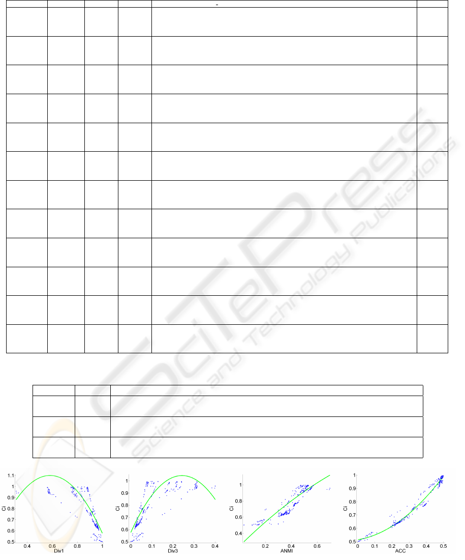
Table 1: Average C

∗

, P

) percentage values obtained by EAC, JWEACS and SWEACS for Optdigits data set.

CE Ext. Alg. EAC JWEAC HubN Dunn S Dbw CH S I XB DB SD PS C. Step

KM 39.75 34.47 36.89 36.66 38.14 35.29 10.00 39.16 38.03 33.84 42.09 33.55 34.19

SL 10.60 10.60 10.60 10.60 10.60 10.60 10.10 10.60 10.60 10.60 10.60 10.60 11.19

AL 10.60 10.60 10.60 10.60 10.60 10.60 10.10 10.60 10.60 10.60 10.60 10.60 20.21

WR 40.31 40.31 40.53 40.30 40.40 40.31 10.10 40.30 40.31 40.40 40.49 40.31 44.28

KM 70.33 69.84 71.09 68.83 70.40 71.47 70.42 72.19 69.59 67.68 69.49 68.83 73.93

SL 60.14 60.21 60.14 60.14 51.48 60.37 60.14 60.37 60.14 60.14 60.14 60.14 67.65

AL 67.29 67.28 67.29 67.29 67.29 67.30 67.29 69.42 67.28 67.29 67.29 67.29 67.28

WR 82.10 82.06 82.10 82.10 83.57 84.31 82.10 84.31 82.10 82.10 82.10 82.09 84.32

KM 62.77 62.39 64.20 63.05 62.28 64.97 64.82 66.30 62.97 63.78 68.95 62.92 64.25

SL 53.76 52.54 53.80 53.80 53.80 58.45 58.57 58.25 52.72 53.80 52.47 52.52 58.15

AL 69.28 70.97 70.94 70.94 69.28 70.89 71.21 63.50 69.28 70.94 70.94 70.94 70.53

WR 76.27 76.34 76.35 76.27 76.27 71.16 76.35 71.14 76.34 76.26 76.35 76.35 71.25

KM 68.77 69.43 72.56 69.97 73.75 73.43 69.52 70.94 69.57 69.29 71.81 74.39 67.86

SL 30.59 30.60 30.21 30.60 30.78 30.21 30.78 30.69 30.78 30.60 30.60 30.60 59.50

AL 79.78 79.43 79.42 79.51 79.32 77.49 79.41 77.54 79.41 79.78 79.41 79.60 79.35

WR 79.51 79.67 79.49 79.85 79.71 77.11 78.85 77.00 78.74 78.97 78.87 79.75 78.05

CLARANS

KM 63.96 63.61 65.60 65.24 65.39 67.14 64.58 65.13 62.32 65.69 62.28 65.38 62.81

SL 20.31 20.11 20.31 20.51 20.51 19.81 20.31 19.81 20.40 20.31 20.31 20.31 42.67

AL 82.73 82.37 82.24 82.78 82.48 75.53 81.11 75.32 82.60 82.21 82.85 79.34 76.15

WR 78.85 78.66 79.27 79.25 77.54 78.58 79.37 78.81 79.06 78.86 77.12 79.27 77.37

ALL5

KM 71.49 69.85 69.52 69.93 69.43 71.31 69.67 70.70 75.98 70.57 69.11 67.77 64.77

SL 39.50 30.30 49.24 30.30 20.81 40.40 49.83 40.39 30.39 20.60 30.30 30.30 51.23

AL 65.57 65.22 73.21 51.24 30.50 71.14 80.44 65.62 60.11 30.41 30.60 30.79 65.32

WR 80.86 80.88 80.51 80.89 80.76 80.95 80.54 80.98 80.53 80.31 80.69 80.51 80.85

CHM

KM 71.97 72.12 73.11 71.40 73.74 72.17 72.69 72.77 73.20 70.48 72.26 73.10 68.74

SL 62.44 62.24 62.06 62.43 62.62 62.63 62.63 61.66 62.61 62.44 62.24 62.24 78.34

AL 87.14 86.88 86.53 87.28 86.46 87.28 87.31 86.76 86.26 86.75 86.82 86.50 84.78

WR 87.54 87.74 87.61 87.51 87.53 87.78 87.52 87.72 87.56 87.68 87.76 87.91 88.03

CLIQUE

KM 59.41 60.29 61.33 59.84 59.95 60.69 63.27 61.28 61.90 60.50 60.41 60.30 64.19

SL 10.50 10.47 10.50 10.48 10.48 10.50 10.47 10.49 10.50 10.48 10.48 10.50 18.76

AL 61.03 63.30 64.89 62.20 62.13 63.67 65.71 64.12 66.02 63.65 63.29 64.54 62.85

WR 67.00 68.23 69.11 67.65 67.68 68.77 73.19 71.02 71.36 69.30 68.67 69.03 70.69

CURE

KM 58.84 57.03 62.75 58.15 45.17 66.12 23.81 51.28 50.60 55.22 52.17 46.88 63.06

SL 10.63 10.63 10.63 10.63 10.62 10.62 16.61 10.64 10.63 10.63 10.63 10.63 11.00

AL 10.60 10.60 10.58 10.60 10.61 10.63 18.39 10.61 10.60 10.61 10.61 10.60 26.81

WR 67.09 67.04 75.55 68.00 62.29 77.48 26.16 71.46 63.41 65.81 63.82 63.56 71.25

DBSCAN

KM 68.81 69.61 70.18 67.85 66.97 69.71 68.68 68.51 69.42 69.04 69.51 70.00 71.10

SL 62.87 62.56 63.01 63.15 62.72 64.40 62.52 65.09 63.88 63.16 62.86 63.20 75.86

AL 77.21 77.16 77.07 77.11 76.76 76.90 77.16 77.25 76.69 77.20 76.85 76.88 77.32

WR 80.98 79.84 80.02 80.36 81.06 79.13 80.78 78.82 78.83 80.61 79.96 79.36 81.19

STING

KM 60.60 59.77 59.00 59.49 60.27 60.09 58.60 59.01 58.70 59.17 59.47 58.55 62.07

SL 22.03 22.03 22.17 22.05 21.99 22.59 19.59 23.71 22.50 22.01 22.01 22.02 34.97

AL 37.89 38.01 37.86 38.07 36.32 39.97 46.09 42.06 37.97 36.72 37.60 37.60 48.40

WR 57.65 57.74 57.90 57.60 57.66 57.69 66.12 57.77 57.72 57.64 57.70 57.63 58.35

ALL10

KM 72.36 72.05 72.50 72.64 72.04 71.40 72.33 72.36 72.62 73.39 72.96 73.67 66.39

SL 42.66 38.14 53.57 32.91 20.63 55.39 55.24 49.65 30.82 20.47 30.20 30.21 59.59

AL 74.22 70.63 74.95 61.66 22.04 76.03 83.09 75.23 62.20 30.59 30.23 31.40 73.58

WR 83.24 83.87 83.65 83.80 83.83 83.14 83.78 82.89 84.14 83.54 84.19 83.69 83.10

Table 2: Average and best C

∗

, P

) percentage values obtained by EAC, JWEACS and SWEACS for all data sets.

Approach Bars Breast Cigar Half Rings Iris Log Yeast Optical Std Yeast Spiral

EAC

Average 86.80 80.96 85.57 84.13 73.88 34.14 58.33 53.23 67.22

Best 99.50 97.07 100.00 100.00 97.37 40.93 87.54 88.50 100.00

SWEACS

Average 84.65 80.58 84.23 83.10 74.30 33.97 57.25 54.00 65.83

Best 99.50 97.08 100.00 100.00 97.19 41.57 87.74 90.89 100.00

JWEACS

Average 86.98 80.38 84.66 83.96 74.59 34.16 57.83 53.80 66.57

Best 99.50 97.20 100.00 100.00 97.29 41.58 87.91 92.64 100.00

Figure 3: Ci vs each cluster ensemble selection measures for Bars data set.

CLUSTER ENSEMBLE SELECTION - Using Average Cluster Consistency

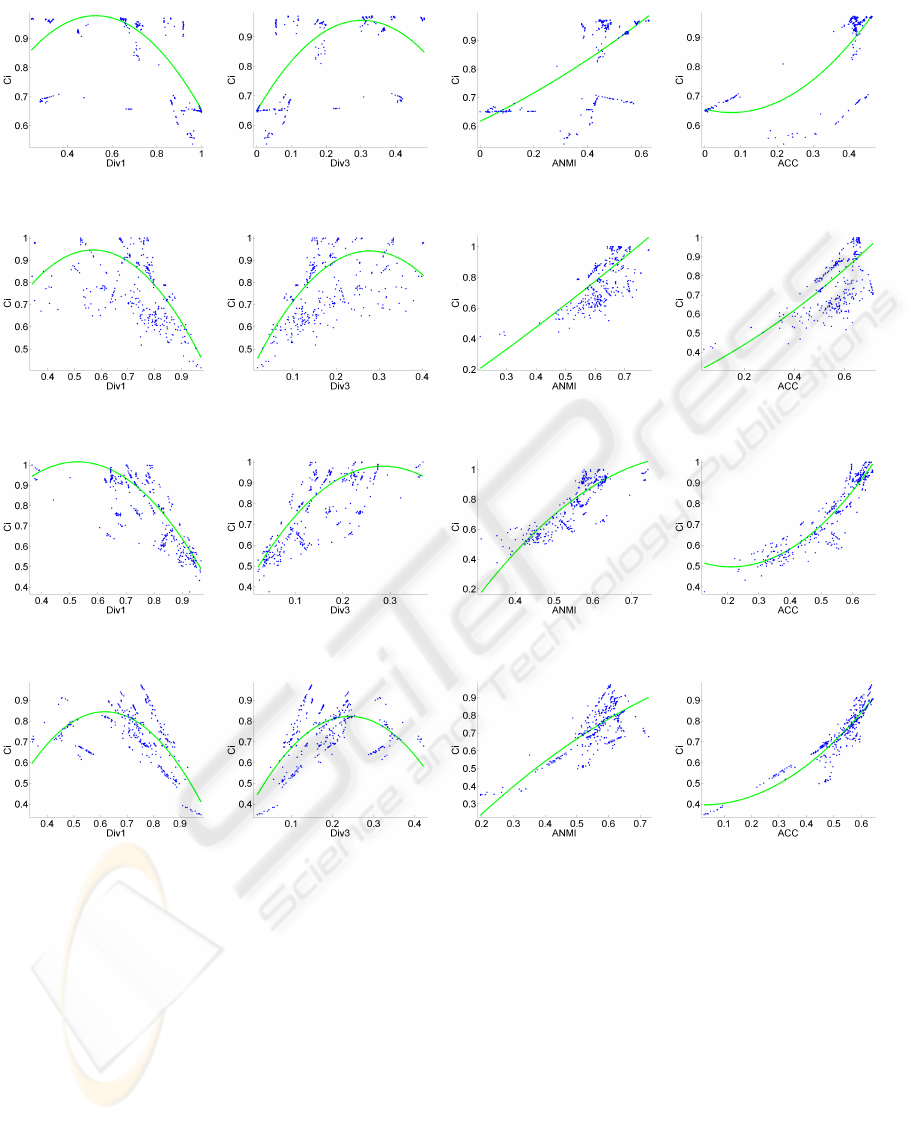
Figure 4: Ci vs each cluster ensemble selection measures for Breast Cancer data set.

Figure 5: Ci vs each cluster ensemble selection measures for Cigar data set.

Figure 6: Ci vs each cluster ensemble selection measures for Half Rings data set.

Figure 7: Ci vs each cluster ensemble selection measures for Iris data set.

The ANMI and ACC measures also do not show a

clear correlation with C

. However, in both plots, one

can see a cloud of points that indicates some correla-

tion between the measures and the Consistency index,

specially in the ACC plot.

In ﬁgure 9, the results of the cluster ensemble se-

lection methods for Std Yeast data set are presented.

Once again, there is no clear correlation between Div

and Div

measures and the C

values. The ANMI and

ACC measures also do not present such correlation.

However, there is a weak tendency of clustering qual-

ity improvement as these measures values increase.

In the Optdigits data set, all measures are corre-

lated with the quality of the consensus partitions. This

correlation is stronger in ACC measure, as it can be

seen in ﬁgure 10. The values of Div

decrease as

the clustering quality is improved while the quality

of the consensus partitions is improved as the values

of Div

, ANMI and ACC measures increase.

The plots for the last data set, Spiral, are presented

in ﬁgure 11. The Div

and Div

measures do not

present correlation with C

values, while the ANMI

and ACC measures show weak tendencies of cluster-

ing improvement with the increasing of their values,

specially in ACC cluster ensemble selection measure.

Table 3 shows the correlation coefﬁcients between

the Consistency index and the consensus partition se-

lection measures. Values close to 1 (-1) suggest that

KDIR 2009 - International Conference on Knowledge Discovery and Information Retrieval

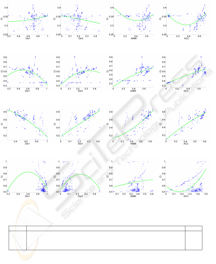
Figure 8: Ci vs each cluster ensemble selection measures for Log Yeast data set.

Figure 9: Ci vs each cluster ensemble selection measures for Std Yeast data set.

Figure 10: Ci vs each cluster ensemble selection measures for Optdigits data set.

Figure 11: Ci vs each cluster ensemble selection measure for Spiral data set.

Table 3: Correlation coefﬁcients between the Consistency index (Ci) and the consensus partition selection measures (Div

Div

, ANMI and ACC measures) for each data set.

Measure Bars Breast C. Cigar Half Rings Iris Log Yeast Std Yeast Optdigits Spiral Average

Div1 -0.5712 -0.6006 -0.3855 -0.6444 -0.3010 0.2448 -0.5356 -0.7922 0.0044 -0.3979

Div3 0.6266 0.6487 0.4367 0.6838 0.2578 -0.2820 0.5450 0.7123 0.0450 0.4082

ANMI 0.8635 0.7979 0.6293 0.8480 0.6856 -0.0444 0.7141 0.7785 0.1095 0.5980

ACC 0.8480 0.8684 0.6154 0.9308 0.8785 -0.0897 0.8505 0.9149 0.4187 0.6928

there is a positive (negative) linear relationship be-

tween Ci and the selection measure, while values

close to 0 indicate that there is no such linear re-

lationship. In 6 out of the 9 data sets used in the

experiments, the ACC measure obtained the highest

linear relationship with the clustering quality (mea-

sured using the Consistency index). In the other 3

data sets, the highest linear relationships were ob-

tained by the ANMI measure in the Bars (0.8635

against 0.8480 achieved by ACC) and Cigar (0.6293

against 0.6154 achieved by ACC) data sets, and by

the Div

measure in the Log Yeast data set which

CLUSTER ENSEMBLE SELECTION - Using Average Cluster Consistency

Table 4: Ci values for the consensus partition selected by Div

, Div

, ANMI and ACC measures, and the maximum C

value

obtained, for each data set.

Measure Bars Breast C. Cigar Half Rings Iris Log Yeast Std Yeast Optdigits Spiral Average

Div1 95.47 95.11 97.93 99.90 87.35 26.96 57.97 58.55 51.68 74.54

Div3 99.50 95.38 100.0 100.0 85.12 29.92 67.66 30.60 51.94 73.35

ANMI 95.75 96.92 97.85 100.0 68.04 35.42 69.09 84.31 51.63 77.67

ACC 99.50 97.07 70.97 95.20 90.67 35.61 53.99 84.31 100.0 80.81

Max Ci 99.50 97.20 100.0 100.0 97.37 41.57 92.64 88.03 100.0 90.70

achieved −0.2820, a counterintuitive correlation co-

efﬁcient when observing the positive coefﬁcients ob-

tained by Div

for all the other data sets. In aver-

age, the ACC measure presents the highest linear re-

lationship with Ci (0.6928), followed by the ANMI

(0.5980), Div

(0.4082) and Div

(-0.3979) measures.

Table 4 presents the Consistency index values

achieved by the consensus partitions selected by

the cluster ensemble selection measures (Div

, Div

ANMI and ACC) for each data set, the maximum C

value of all the produced consensus partitions and the

average C

values for each best consensus partition se-

lection measure. The consensus partitions for Div

and Div

measures were selected choosing the con-

sensus partition corresponding to the median of their

values, as mentioned in (Hadjitodorov et al., 2006).

For the ANMI and ACC measures, the best consensus

partition was selected to be the one that maximizes the

respective measures.

The quality of the consensus partitions selected

by ACC measure was in 6 out of 9 data sets supe-

rior or equal to the quality of the consensus partitions

selected by the other measures, speciﬁcally, in Bars

(99.50%), Breast Cancer (97.07%), Iris (90.67%),

Log Yeast (35.61%), Optdigits (84.31%) and Spiral

(100%) data sets. In Cigar data set, the best consensus

partition was selected using Div

measure (100%),

and the same happened in Half Rings data set to-

gether with ANMI. In Std Yeast data set, none of

the four measures selected a consensus partition with

similar quality to the best produced consensus parti-

tion (92.64%). The closed selected consensus parti-

tion was selected using ANMI (69.09%). Concern-

ing the average quality of the partitions chosen by the

four measures, the ACC measure stands out again,

achieving 80.81% of accuracy, followed by ANMI

with 77.67%. The Div

and Div

measures obtained

the worst performance with 74.54% and 73.35%, re-

spectively.

6 CONCLUSIONS

This paper adresses the problem of selecting the best

consensus partition from a set of consensus parti-

tions, that best ﬁts a given data set. The motiva-

tion of this work is related to the variety of methods

that can be used to produce the multiple data parti-

tions in a cluster ensemble and to the different con-

sensus function that can be applied to combine them

and produce a more robust consensus data partition.

We used the Evidence Accumulation Clustering and

the Weighted Evidence Accumulation Clustering us-

ing Subsampling combination approaches to illustrate

the diversity in the quality of the resulting consensus

partitions, and thus, the need to select a good consen-

sus partition among all the produced consensus parti-

tions. We proposed the Average Cluster Consistency

(ACC) measure to select the best consensus partition

for a given data set, based on a new similarity notion

between each data partition belonging to the cluster

ensemble and a given consensus partition.

Experiments using 9 different data sets were car-

ried out in order to assess the performance of the pro-

posed cluster ensemble selection method. The exper-

imental results presented in this paper show that the

ACC measure is the best consensus partition selection

measure when compared to other three measures, and

thus a good option for selecting a high quality con-

sensus partition from a set of consensus partitions.

REFERENCES

Agrawal, R., Gehrke, J., Gunopulos, D., and Raghavan, P.

(1998). Automatic subspace clustering of high dimen-

sional data for data mining applications. SIGMOD

Rec., 27(2):94–105.

Calinski, R. (1974). A dendrite method for cluster analysis.

Communications in statistics, 3:1–27.

Chou, C., Su, M., and Lai, E. (2004). A new cluster valid-

ity measure and its application to image compression.

Pattern Analysis and Applications, 7:205–220.

Davies, D. and Bouldin, D. (1979). A cluster separation

measure. IEEE Transaction on Pattern Analysis and

Machine Intelligence, 1(2).

Duarte, F. J., Fred, A. L. N., Rodrigues, M. F. C., and

Duarte, J. (2006). Weighted evidence accumulation

clustering using subsampling. In Sixth International

Workshop on Pattern Recognition in Information Sys-

tems.

KDIR 2009 - International Conference on Knowledge Discovery and Information Retrieval

Dunn, J. (1974). Well separated clusters and optimal fuzzy

partitions. J. Cybern, 4:95–104.

Ester, M., Kriegel, H.-P., J

org, S., and Xu, X. (1996).

A density-based algorithm for discovering clusters in

large spatial databases with noise.

Fern, X. and Brodley, C. (2004). Solving cluster ensem-

ble problems by bipartite graph partitioning. In ICML

’04: Proceedings of the twenty-ﬁrst international con-

ference on Machine learning, page 36, New York, NY,

USA. ACM.

Fred, A. L. N. (2001). Finding consistent clusters in data

partitions. In MCS ’01: Proceedings of the Second In-

ternational Workshop on Multiple Classiﬁer Systems,

pages 309–318, London, UK. Springer-Verlag.

Fred, A. L. N. and Jain, A. K. (2005). Combining multiple

clusterings using evidence accumulation. IEEE Trans.

Pattern Anal. Mach. Intell., 27(6):835–850.

Guha, S., Rastogi, R., and Shim, K. (1998). Cure: an ef-

ﬁcient clustering algorithm for large databases. In

SIGMOD ’98: Proceedings of the 1998 ACM SIG-

MOD international conference on Management of

data, pages 73–84, New York, NY, USA. ACM.

Hadjitodorov, S. T., Kuncheva, L. I., and Todorova, L. P.

(2006). Moderate diversity for better cluster ensem-

bles. Inf. Fusion, 7(3):264–275.

Halkidi, M., Batistakis, Y., and Vazirgiannis, M. (2001).

Clustering algorithms and validity measures. In Tu-

torial paper in the proceedings of the SSDBM 2001

Conference.

Hubert, L. and Arabie, P. (1985). Comparing partitions.

Journal of Classiﬁcation.

Hubert, L. and Schultz, J. (1975). Quadratic assignment

as a general data-analysis strategy. British Journal

of Mathematical and Statistical Psychology, 29:190–

241.

Jouve, P. and Nicoloyannis, N. (2003). A new method

for combining partitions, applications for distributed

clustering. In International Workshop on Paralell

and Distributed Machine Learning and Data Mining

(ECML/PKDD03), pages 35–46.

Karypis, G., Eui, and News, V. K. (1999). Chameleon: Hi-

erarchical clustering using dynamic modeling. Com-

puter, 32(8):68–75.

Kaufman, L. and Roussesseeuw, P. (1990). Finding groups

in data: an introduction to cluster analysis. Wiley.

King, B. (1973). Step-wise clustering procedures. Journal

of the American Statistical Association, (69):86–101.

Kuncheva, L. and Hadjitodorov, S. (2004). Using diver-

sity in cluster ensembles. volume 2, pages 1214–1219

vol.2.

Macqueen, J. B. (1967). Some methods of classiﬁcation

and analysis of multivariate observations. In Proceed-

ings of the Fifth Berkeley Symposium on Mathemtical

Statistics and Probability, pages 281–297.

Maulik, U. and Bandyopadhyay, S. (2002). Performance

evaluation of some clustering algorithms and validity

indices. IEEE Transactions on Pattern Analysis and

Machine Intelligence, 24(12):1650–1654.

Ng, R. T. and Han, J. (2002). Clarans: A method for clus-

tering objects for spatial data mining. IEEE Trans. on

Knowl. and Data Eng., 14(5):1003–1016.

Sneath, P. and Sokal, R. (1973). Numerical taxonomy. Free-

man, London, UK.

Strehl, A. and Ghosh, J. (2003). Cluster ensembles — a

knowledge reuse framework for combining multiple

partitions. J. Mach. Learn. Res., 3:583–617.

Topchy, A., Jain, A. K., and Punch, W. (2003). Combining

multiple weak clusterings. pages 331–338.

Topchy, A., Minaei-Bidgoli, B., Jain, A. K., and Punch,

W. F. (2004a). Adaptive clustering ensembles. In

ICPR ’04: Proceedings of the Pattern Recognition,

17th International Conference on (ICPR’04) Volume

1, pages 272–275, Washington, DC, USA. IEEE Com-

puter Society.

Topchy, A. P., Jain, A. K., and Punch, W. F. (2004b). A mix-

ture model for clustering ensembles. In Berry, M. W.,

Dayal, U., Kamath, C., and Skillicorn, D. B., editors,

SDM. SIAM.

Wang, W., Yang, J., and Muntz, R. R. (1997). Sting: A sta-

tistical information grid approach to spatial data min-

ing. In VLDB ’97: Proceedings of the 23rd Interna-

tional Conference on Very Large Data Bases, pages

186–195, San Francisco, CA, USA. Morgan Kauf-

mann Publishers Inc.

Ward, J. H. (1963). Hierarchical grouping to optimize an

objective function. Journal of the American Statistical

Association, 58(301):236–244.

Xie, X. and Beni, G. (1991). A validity measure for fuzzy

clustering. IEEE Transactions on Pattern Analysis

and Machine Intelligence, 13:841–847.

CLUSTER ENSEMBLE SELECTION - Using Average Cluster Consistency