
ITEM-USER PREFERENCE MAPPING WITH MIXTURE MODELS
Data Visualization for Item Preference
Yu Fujimoto
Dept. Integrated Information Technology, Aoyama Gakuin Univ., Kanagawa, Japan
Hideitsu Hino, Noboru Murata
Dept. Electrical Engineering and Bioscience, Waseda Univ., Tokyo, Japan
Keywords:
Bradley-Terry model, Mixture model, EM algorithm, Preference map, Data visualization.
Abstract:
In this paper, we propose a visualization technique of a statistical relation of users and preference of items
based on a mixture model. In our visualization, items are given as points in a few dimensional preference
space, and user specific preferences are given as lines in the same space. The relationship between items and
user preferences are intuitively interpreted via projections from points onto lines. As a primitive implementa-
tion, we introduce a mixture of the Bradley-Terry models, and visualize the relation between items and user
preferences with benchmark data sets.
1 INTRODUCTION
In a market research study or an item recommenda-
tion system, it is very important to model and inter-
pret a statistical relation of “users” and “preference of
items” based on a data set. Visualization of such mod-
els helps us to discover new relations between items
and users, e.g. unknown preference tendency for a
specific user. And visualization also supports to inter-
pret results of item recommendation in systems.
It has an old history to model preference levels
of items from the statistical aspect. Most researchers
assume that a preference parameter θ
i
is attached to
the item T
i
for I different items (Bradley and Terry,
1952; Luce, 1959; Plackett, 1975). With this param-
eter, favorable or unfavorable items for users are in-
tuitively interpreted. However, the preference param-
eter potentially has absurdity, because it is obtained
based on data which reflect various users’ average,
and the one-dimensional preference assumption may
cause a wrong interpretation. Then, an idea of mul-
tiple preferences, which is an assumption that a user
evaluates an item comprehensively with some indices
such as one’s interest and credibility of the item, is
naturally introduced. For representation of multiple
preferences, some applications of mixture models are
proposed (Croon and Luijkx, 1993; Murphy and Mar-
tin, 2003).
In this paper, we propose a visualization of re-
lation between items and users to assist analysis of
multiple preferences based on mixture models. In our
visualization, items are mapped in a K-dimensional
space associated with K preference coordinates and
their levels on a user specific preference are shown
as projections onto a line on the map. With this map-
ping, preference relation between items and user pref-
erences can be visually interpreted.
This paper is composed as follows. In Section 2,
a simple probability model with preference parame-
ters, broadly known as the Bradley-Terry (BT) model,
and its mixtures are introduced. In Section 3, an
idea for preference mapping which visualizes the item
preference is explained. We also mention differences
among other visualization tools and our method. Sec-
tion 4 shows experimental results of the item prefer-
ence mapping based on mixtures of BT models. And
Section 5 is devoted to concluding remarks.
2 PREFERENCE MODEL AND
ITS MIXTURE
Let T
i
be the i-th item where i = 1, . . . , I. Here, a pref-
erence parameter set θ = {θ
1
, . . . , θ
I
} is introduced to
represent relative preference levels for I items. Statis-
105
Fujimoto Y., Hino H. and Murata N. (2009).
ITEM-USER PREFERENCE MAPPING WITH MIXTURE MODELS - Data Visualization for Item Preference.
In Proceedings of the International Conference on Knowledge Discovery and Information Retrieval, pages 105-111
DOI: 10.5220/0002274001050111
Copyright
c
SciTePress

tical models denoted with such a preference parame-
ter set are called preference models in this paper. We
introduce a simple preference model, the BT model
(Bradley and Terry, 1952), and its mixture.
2.1 Bradley-Terry Model
Assume that a user evaluates two items T
i
and T
j
with
ratings r
i
, r
j
∈ N, and each user chooses a preferred
item from T
i
and T
j
by comparing r
i
and r
j
. Let
T
i
≻ T
j
be the event r
i
> r
j
, which indicates that T
i
is chosen in the comparison of T
i
and T
j
, and X
ij
be a
variable for the comparison result which takes one of
{T
i
≻ T
j
, T
j
≻ T
i
}. In the BT model, the probability
that “the item T
i
is preferred in the comparison of T
i
and T
j
”, denoted as p(T
i
≻ T
j
;θ), is given by
p(T
i
≻ T
j
;θ) =
θ
i
θ
i
+ θ
j
(i 6= j), (1)
where
I
∑
i=1
θ
i
= 1, θ
i
> 0 (i = 1, . . ., I).
Intuitively speaking, the item T
i
which has larger θ
i
is chosen more frequently, and θ indicates a set of
preference levels which is common to N users.
Let X
n
= {X
n
ij
|1 ≤i < j ≤I}be all the paired com-
parisons in I items, compared by the n-th user. Under
the assumption that each comparison is independent,
the probability Pr(X
n
= x
n
) = p(x
n
;θ), where x
n
is an
observation from the n-th user, is given by
p(x
n
;θ) =
∏
i6= j
θ
i
θ
i
+ θ
j
c
n
ij
, (2)
where c
n
ij
is an indicator, that is
(c
n
ij
, c
n
ji
) =
(1, 0) (x
n
ij
= T
i
≻ T
j
)
(0, 1) (x
n
ij
= T
j
≻ T
i
)
(0, 0) (x
n
ij
is missed).
(3)
Note that (c
n
ij
, c
n
ji
) = (0, 0) indicates that the compar-
ison x
n
ij
is missed because the items T
i
or/and T
j
are
not rated, or their ratings are the same
1
.
With Eq.(2), the log likelihood of x
1:N
=
{x
1
, . . . , x
N
} is given as follows,
L(θ) =
N
∑
n=1
log p(x
n
;θ) =
N
∑
n=1
∑
i6= j
c
n
ij
log
θ
i
θ
i
+ θ
j
=
∑
i6= j
c
ij
log
θ
i
θ
i
+ θ
j
, (4)
1
The modeling of paired comparison data with ties (r
i
=
r
j
) also has a long history (Rao and Kupper, 1967; Davidson
and Beaver, 1977; Joe, 1990; Kuk, 1995), though tied cases
are neglected for simplicity in this paper.
where c
ij
=
∑
N
n=1
c
n
ij
.
The maximum likelihood (ML) estimation proce-
dure for the BT model, which achieves
ˆ
θ = argmax
θ
∑
i6= j
c
ij
log
θ
i
θ
i
+ θ
j
, (5)
has been already discussed from several contexts, and
some iterative estimation methods for the ML esti-
mator
ˆ
θ have been introduced (Hastie and Tibshirani,
1998; Huang et al., 2006). In this paper, the estima-
tion is achieved by the following algorithm used in
Huang et al.(2006).
Algorithm 1. Estimation of BT model.
input pairwise comparison data x
1:N
.
initialize t = 0, and choose an initial parameter θ
(0)
.
repeat until convergence
update
θ
(t+1)
i
←
∑
j6=i
c
ij
∑
j6=i
c
ij
+c
ji
θ
(t)
i
+θ
(t)
j
, (6)
for i = 1, . . . , I.
normalize θ
(t+1)
and set t ← t + 1.
output converged parameter vector θ.
2.2 Mixture Model
In the previous subsection, the BT model was ex-
plained. In this subsection, a mixture of BT models
and its estimation method are introduced.
We assume that “users evaluate items based on K
preference parameter sets with their own weights“,
and introduce a mixture model whose component re-
spectively represents a preference from a different
point of view. Under this assumption, the distribution
of X
n
is given by the mixture of preference models,
p(X
n
) =
K
∑
k=1
p(M
k
)p(X
n
|M
k
), (7)
where M
k
is the k-th preference model with the pa-
rameter set θ
k
= {θ
k
1
, . . . , θ
k
I
} and p(X
n
|M
k
) is given
by Eq.(2) with the parameter set θ
k
. And the log like-
lihood for x
1:N
is given as
L(Θ) =
N
∑
n=1
log
K
∑
k=1
p(M
k
)p(x
n
|M
k
), (8)
where Θ = {θ
1
, . . . , θ
K
} is the set of parameters for
the mixture.
Since the direct maximization of Eq.(8) is com-
plex, we apply the EM algorithm (McLachlan and Kr-
ishnan, 1996) to estimate the mixture of BTs. The ob-
jective function, so-called the Q-function, for the EM
KDIR 2009 - International Conference on Knowledge Discovery and Information Retrieval
106

estimation is defined as follows,
Q(Θ;Θ
(t)
)
=
N
∑
n=1
K
∑
k=1
p(M
k
|x
n
;Θ
(t)
)log p(x
n
|M
k
;Θ) (9)
=
N
∑
n=1
K
∑
k=1
p(M
k
|x
n
;Θ
(t)
)
∑
i6= j
c
n
ij
log
θ
k
i
θ
k
i
+ θ
k
j
=
K
∑
k=1
∑
i6= j
w
k(t)
ij
log
θ
k
i
θ
k
i
+ θ
k
j
, (10)
where w
k(t)
ij
=
∑
N
n=1
c
n
ij
p(M
k
|x
n
;θ
k(t)
). We call
p(M
k
|x
n
) user weight. With this function, a procedure
for the EM estimation is denoted as follows.
Algorithm 2. The EM estimation.
input pairwise comparison data x
1:N
.
initialize t = 0, and choose an initial parameter Θ
(0)
repeat until convergence
E-step: calculate user weight p(M
k
|x
n
;Θ
(t)
) of Eq.(9)
by
p(M
k
|x
n
;Θ
(t)
) =
∏
i6= j
c
n
ij
θ
k(t)
i
θ
k(t)
i
+θ
k(t)
j
∑
K
m=1
∏
i6= j
c
n
ij
θ
m(t)
i
θ
m(t)
i
+θ
m(t)
j
. (11)
M-step: maximize the Q-function given by Eq.(10)
with respect to Θ, that is equivalent to
θ
k(t+1)
= argmax
θ
k
∑
i6= j
w
k(t)
ij
log
θ
k
i
θ
k
i
+ θ
k
j
(12)
for all k, and set t ←t + 1.
output converged parameter vector
ˆ
Θ.
Note that Eq.(12) is equivalent to Eq.(5) and the
maximization is achieved based on Algorithm 1 by
using w
k(t)
ij
instead of c
ij
. As broadly known, the EM
algorithm is the local maxima algorithm. In our ex-
periments, therefore, models are estimated five times
from randomly chosen initial parameters, and the one
which achieves the highest Q-value is used.
For selection of the optimal K, the information cri-
teria (Akaike, 1974; Barron et al., 1998) or cross val-
idation (CV)(Hastie et al., 2001) are applicable. In
Section 4, we use CV to select K.
3 PREFERENCE MAPPING
As defined in Section 2, preference models have pa-
rameters to represent preferences for I items. With
0.0 0.1 0.2 0.3 0.4 0.5
T1
T2
T3
T4
T5
√
θ
Figure 1: An example of preference mapping in one-
dimensional case. Items are plotted according to the square
root of θ to facilitate visualization.
o
o
o
o
o
o
o
o
o
o
o
o
o
o
o
0.0 0.2 0.4 0.6 0.8 1.0
0.0 0.2 0.4 0.6 0.8 1.0
T 1
T 2
T 3
T 4
T 5
√
θ
1
√
θ
2
Figure 2: An example of 2D preference mapping.
a mixture of K preference models, an item T
i
can
be mapped on a K-dimensional space and its coor-
dinate (θ
1
i
, . . . , θ
K
i
) gives us an intuitive interpretation
of preference relation. In this section, we propose an
intuitive preference mapping tool based on a mixture
model.
3.1 Item Mapping
By introducing a preference model, the preference
tendency of each item is interpreted intuitively by
plotting the parameter on an axis. Figure 1 shows an
example of such a plot. It is visually understood that
T
4
tends to be preferred as shown in the figure. We
call this type of plot a preference map
2
.
In the case of a mixture model, θ
k
shows one of
the K coordinates for representation of preference lev-
els. Accordingly, the multiple preference parameters
with K ≥ 2 can be mapped in a K-dimensional space
in the same way. Figure 2 shows an example of two-
dimensional preference mapping of I = 15 items. On
a 2D preference map, those items which are com-
monly preferred by various users, like T
4
, are mapped
on the upper right side in the figure, and not preferred
items in one dimension are mapped near the other
axis, like T
2
and T
3
.
2
In this paper, all the axes in preference maps are given
in the square root of preference parameters for easy-to-see
visualization though it is not essential.
ITEM-USER PREFERENCE MAPPING WITH MIXTURE MODELS - Data Visualization for Item Preference
107

o
o
o
o
o
o
o
o
o
o
o
o
o
o
o
0.0 0.2 0.4 0.6 0.8 1.0
0.0 0.2 0.4 0.6 0.8 1.0
T 1
T 2
T 3
T 4
T 5
√
θ
1
√
θ
2
Figure 3: Preference mapping in a 2D space. A solid line
in the map shows a user preference weight and dotted lines
show projections onto the user preference levels which in-
dicates φ
n
.
0.0 0.1 0.2 0.3 0.4 0.5
T1
T2
T3
T4
T5
√
φ
n
Figure 4: An example of a user preference φ
n
. Plots are
corresponding to the projected items onto the line in Figure
3.
3.2 User Preference
As previously denoted, we assume that “users evalu-
ate items based on K preference parameter sets with
their own weights” for the mixture model, and a
user preference weight can be shown as a vector
(p(M
1
|x
n
), . .. , p(M
K
|x
n
)) in a preference map. The
direction of this vector expresses that the user thinks
which coordinate is more important. For example, the
solid line in Figure 3 shows a user preference weight
for the user n which has tangents of
p(M
2
|x
n
)
p(M
1
|x
n
)
. The line
indicates that the user rely on both of the axes θ
1
and
θ
2
.
Additionally, we can obtain a user specific prefer-
ence levels {φ
n
i
} of {T
i
} by projecting items onto the
line on the map. Figure 3 also shows an example of
item projections given as dotted lines to represent user
preference levels. Projected points on the line indicate
us the one-dimensional preference levels for the n-th
user (see, Figure 4) embedded in the K-dimensional
space. Such a projection can be expressed with the
coordinate of T
i
and the user preference weight. For
example, one can easily come up with a projection
given by the simple mixture of K parameters: a level
of T
i
on the n-th user preference is given by
φ
n
i
=
K
∑
k=1
p(M
k
|x
n
)θ
k
i
. (13)
Projection defined by Eq.(13) is called linear projec-
tion in this paper. For another example, a projection
given by the mixture of K parameters in a sense of the
single BT estimation is also possible, that is given by
φ
n
= argmax
φ
n
∑
j6=l
K
∑
k=1
p(M
k
|x
n
)
θ
k
j
θ
k
j
+ θ
k
l
!
log
φ
n
j
φ
n
j
+ φ
n
l
,
(14)
where φ
n
= {φ
n
1
, . . . , φ
n
I
}. We call projection defined
by Eq.(14) BT projection. The former type of pro-
jection is very simple however the latter one seems
natural. In Figures 3 and 4, BT projection is applied
to a specific user preference. In Section 4, two types
of projections are compared.
As denoted at the end of previous section, the op-
timal K for the mixture model can be selected by the
model selection procedure. However we still have a
problem for visualizing preference mapping of a spe-
cific user. A visualization of mapped items is quite
simple in the low dimensional case, however, in the
case of K ≥ 4, we have to visualize the high dimen-
sional preference map in the low dimensional space.
Here, user weight p(M
k
|x
n
) shows that how much the
n-th user emphasizes the k-th preference parameter set
θ
k
. An informative low dimensional preference map
for the user is obtained by picking up some dimen-
sions with the heaviest user weights. Note that the
preferencemap without visualizing dimensions which
have heavy user weights sometimes provides us mis-
leading information. For example, Figure 5 shows an
informative 2D preference map for a user by picking
up θ
2
and θ
3
which havethe two heaviest user weights
in the mixture with K = 4, Figure 6 shows a mislead-
ing 2D preference map for the same user, mapped in
a randomly selected two-dimensional space and Fig-
ure 7 shows the user preference levels φ
n
. In Figure 5,
the mapped items according to preference map coor-
dinates θ
2
and θ
3
roughly reflect the user preference
(φ
n
), e.g. items mapped on the upper right side, like
T
4
, are also highly preferred in Figure 7. By contrast,
items mapped on the upper right side in a misleading
preference map do not preserve this relation, e.g. T
2
in Figure 6 is less preferred than T
4
in φ
n
. Such a con-
flict happens because the low dimensional space with
small p(M
k
|x
n
) does not have valid information about
the n-th user.
3.3 Other Mapping Tools
As a tool for visualization of probabilistic re-
lation between evaluated items and users, the
Multi-Dimensional Scaling (MDS) or the Multi-
Dimensional unfolding (Bennett and Hays, 1960) has
been proposed. Especially the Multi-Dimensional un-
folding is a method to map items and users in a low
KDIR 2009 - International Conference on Knowledge Discovery and Information Retrieval
108
o
o
o
o
o
o
o
o
o
o
o
o
o
o
o
0.0 0.2 0.4 0.6 0.8 1.0
0.0 0.2 0.4 0.6 0.8 1.0
T 1
T 2
T 3
T 4
T 5
√
θ
3
√
θ
2
Figure 5: An example of informative 2D preference map-
ping of the mixture with K = 4.
o
o
o
o
o
o
o
o
o
o
o
o
o
o
o
0.0 0.2 0.4 0.6 0.8 1.0
0.0 0.2 0.4 0.6 0.8 1.0
T 1
T 2
T 3
T 4
T 5
√
θ
4
√
θ
2
Figure 6: An example of misleading preference mapping.
0.0 0.1 0.2 0.3 0.4 0.5
T1
T2
T3
T4
T5
√
φ
n
Figure 7: User preference levels φ
n
corresponding to the
lines in Figure 5 and Figure 6.
dimensional space according to user preference lev-
els of items. Even in recent years, some researchers
also have proposed the preference visualization (Mei
and Shelton, 2006; Zenebe and Norcio, 2007). An ob-
vious difference between their works and ours is the
representation of user preference in the map. In our
method, items are mapped in the K-dimensional space
and their preference levels for each user are given by
projections onto the corresponding line whose direc-
tion indicates the user weight: i.e. how much this user
relies on the axes of the graph relatively. We avoid to
map users and items as points on the same space be-
cause they are not the same kind of data.
To visualize relations between items and user pref-
erences with points and lines, the Arrow and Point
Method (APM) (Hayashi, 1993) has been also pro-
posed. The APM achieves similar mapping as our
method, and also shows the relation between items
and users by points and lines. However the map ob-
tained by our method shows K universal preference
coordinates at the same time and intuitively inter-
preted from a statistical viewpoint, which is a discrim-
inative point that the APM does not have.
4 EXPERIMENTS
In this section, we discuss our visualization method
on real-world data sets. At first, we show the exper-
imental results of tuning the optimal K in a way of
the conventional statistical model selection. Then, we
evaluate a structure of the preference mapping which
is defined by a mixture of preference models from
a viewpoint of precision of user preferences with a
ranking correlation metric.
4.1 Real-world Data Sets
The MovieLens data set is a standard benchmark data
set provided by GroupLens research team (Riedl and
Konstan, 2000). This data set contains 100, 000 rat-
ings answered by N = 943 users for I = 1, 682 movies.
The BookCrossing data set is another benchmark
data set which contains ratings of books (Ziegler
et al., 2005). To obtain dense paired comparison set
for evaluating our preference mapping, we removed
answers rated as 0 and picked up 4, 282 ratings an-
swered by N = 799 users for I = 200 items.
We use these two data sets for evaluation of our
mixture model and preference mapping.
4.2 Evaluation Metric
For a metric of the mapping precision, we use the
ranking correlation between rating data and user pref-
erence levels. Let r
n
i
and r
n
j
be ratings of T
i
and T
j
evaluated by the n-th user. For items evaluated by the
user, if the ordering of r
n
i
and r
n
j
is the same as the
ordering of φ
n
i
and φ
n
j
, a pair (T
i
, T
j
) is called con-
cordant. On the other hand, if the two orderings are
different, the pair is called discordant. In the case of
ties, that is r
n
i
= r
n
j
(or/and φ
n
i
= φ
n
j
), the pair is neither
concordant or discordant. Then the metric is given as
follows
τ
n
b
=
N
n
C
−N
n
D
p
N
n
C
+ N
n
D
+ N
n
r
q
N
n
C
+ N
n
D
+ N
n
φ
, (15)
where N
n
C
(N
n
D
) is the number of concordant (discor-
dant) pairs, and N
n
r
(N
n
φ
) is the number of ties in rat-
ings (preference levels) of the n-th user. Equation (15)
is called Kendall’s tau-b, and used for evaluating the
correlation between two ranking sequences with ties
(Mei and Shelton, 2006). Note that the tau-b metric
ITEM-USER PREFERENCE MAPPING WITH MIXTURE MODELS - Data Visualization for Item Preference
109

1 2 3 4 5
300 400 600
K
negative log likelihood
1 2 3 4 5
1e+04 1e+05 1e+06
K
negative log likelihood
Figure 8: Plots of 5-fold CV results of the negative log
likelihood: left one is the result of BookCrossing data and
right one is that of MovieLens data. The vertical bars in the
graphs show standard deviations.
is −1 ≤ τ
n
b
≤ 1, and τ
n
b
∼
=
1 (τ
n
b
∼
=
−1) indicates the
orderings of the ratings and the user preferences are
strongly positive (negative) correlated. And τ
n
b
= 0
indicates their orderings are independent. Note that
the tau-b metric is calculated between all the pairs of
ratings and user preference levels such that c
n
ij
= 1 for
each user. In the next subsection, we experimentally
show that the mixture of preference models achieves
precise mapping in the viewpoint of the tau-b metric.
4.3 Experimental Results
To visualize preference maps of the BookCrossing
data and the MovieLens data, the optimal K is se-
lected based on 5-fold CV. The results (Figure 8)
showthat K = 2 is selected for both of the BookCross-
ing data and the MovieLens data in the sense of the
one standard deviation rule. Figure 9 shows simpli-
fied distributions of tau-b values between ratings and
user preferences, defined by Eq.(15), of N users. A
user preference φ
n
is calculated under the optimal K
selected by CV (i.e. K = 2) and two types of projec-
tions (linear and BT projections) are applied to derive
φ
n
. And the tau-b values between ratings and θ in the
single BT model is also plotted in Figure 9 for com-
parison. In the figure, mixtures with the both projec-
tions apparently improve tau-b values and the results
show that the mixture organizes more precise prefer-
ence than the single preference model for each user.
In other words, ranking of ratings corresponds to that
of φ
n
on each user preference more specifically by in-
troducing mixture of preference models. The figure
also shows that precision of ranking estimation with
user preference based on the simple linear projection
is approximately the same as that of the BT projec-
tion.
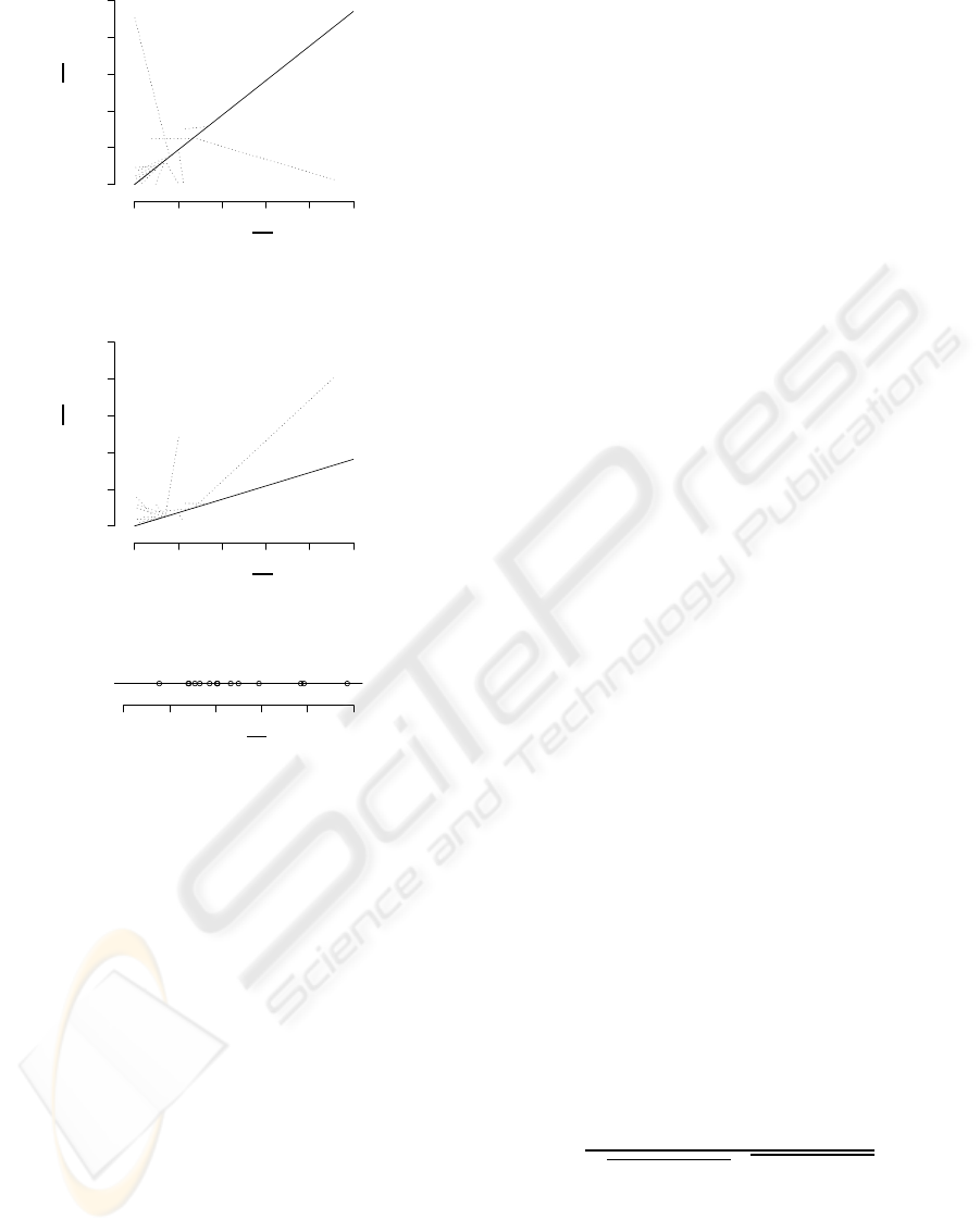
Figure 10 shows 2D preference maps as a result of
the experiment on the BookCrossing data set. The left
figure is the map with a user preference of those who
rely on θ
1
. For such a user, items which have a higher
Single BT
Linear proj.
BT proj.
−0.2 0.0 0.2 0.4 0.6 0.8 1.0
tau−b
Single BT
Linear proj.
BT proj.
0.20 0.25 0.30 0.35 0.40 0.45 0.50
tau−b
Figure 9: Plots of tau-b values. The line in each box indi-
cates the median of tau-b for N users, and the vertical edges
of the box indicate the 75% and 25% quantiles.
value in θ
1
, like T
171
shown as a filled square in the
figure, are attractive (see the upper right figure). On
the other hand, the middle figure is the map with the
index of those who rely on θ
2
. For such a user, an item
like T
55
shown as a filled circle is preferred (see the
lower right). As the result, we can say that preference
maps like Figure 10 has a potential of visualization
which indicates not only relations between items but
also differences between each user preference.
5 CONCLUSIONS AND FUTURE
WORKS
This paper proposes a method to visualize multiple
preferences of items, with a mixture of preference
models. We adopt BT models for simple implementa-
tion of preference model in this paper, while the mix-
ture can be composed of not only BT models but also
any probability models for preference levels. Actu-
ally, as described in Hastie and Tibshirani (1998), the
conventional BT model sometimes leads to the inac-
curate preference parameter θ which does not reflect
the preference order of items. To avoid this prob-
lem, a mixture of modified BT models, such as Huang
et al. (2006), or alternative preference models (Luce,
1959; Plackett, 1975; Hino et al., 2009) should be
applied. We also confirmed that a preference map
can be drawn with other preference models though it
doesn’t explain in this paper. Regardless of whether
BT models are used, the obtained map based on pro-
posed method is directly interpreted as the probability
model, and provides effective suggestions as the anal-
ysis result, e.g. we can show grounds of the recom-
mendation visually for users.
In our method, items are mapped in the K-
dimensional space, user’s preference weights are
KDIR 2009 - International Conference on Knowledge Discovery and Information Retrieval
110

0.0 0.1 0.2 0.3 0.4
0.0 0.1 0.2 0.3 0.4
T55
T171
√
θ
1
√
θ
2
0.0 0.1 0.2 0.3 0.4
0.0 0.1 0.2 0.3 0.4
T55
T171
√
θ
1
√
θ
2
0.00 0.05 0.10 0.15 0.20 0.25
T55
T171
√
φ
n
0.00 0.05 0.10 0.15 0.20 0.25
T55
T171
√
φ
n
Figure 10: Preference maps based on the BookCrossing data set. The left figure shows a user preference of those who rely on
θ
1
, the middle one shows that of those who rely on θ
2
and the right figures show user preference levels φ
n
of these users.
given as lines, and user’s own preference levels are
given by projections onto the corresponding line. We
experimentally compared two types of projections,
linear and BT, and verified that there was no big dif-
ference in results of tau-b metric. As a criterion to vi-
sualize the K-dimensional preference map and a user
preference in a low dimensional space, we focus on
the user weight p(M
k
|x
n
). However, when we com-
pare two users, the low dimensional map which accu-
rately shows difference between their preferences is
expected, though it remains as a future work.
REFERENCES
Akaike, H. (1974). A new look at the statistical model iden-
tification. IEEE Trans. Automatic Control, 19(6):716–
723.
Barron, A., Rissanen, J., and Yu, B. (1998). The minimum
description length principle in coding and modeling.
IEEE Trans. Information Theory, 44(6):2743–2760.
Bennett, J. F. and Hays, W. L. (1960). Multidimensional
unfolding: Determining the dimensionality of ranked
preference data. Psychometrika, 25(1):27–43.
Bradley, R. A. and Terry, M. E. (1952). Rank analysis of in-
complete block designs: I. the method of paired com-
parisons. Biometrika, 39(3/4):324–345.
Croon, M. and Luijkx, R. (1993). Probability Models
and Statistical Analyses for Ranking Data, chapter 4,
pages 53–74. Lecture Notes in Statistics. Springer.
Davidson, R. R. and Beaver, R. J. (1977). On extending the
Bradley-Terry model to incorporate within-pair order
effects. Biometrics, 33(4):693–702.
Hastie, T. and Tibshirani, R. (1998). Classification by pair-
wise coupling. Annals of Statistics, 26(2):451–471.
Hastie, T., Tibshirani, R., and Friedman, J. (2009). The Ele-
ments of Statistical Learning: Data Mining, Inference
and Prediction. 2nd Ed. Springer Series in Statistics.
Springer.
Hayashi, C. (1993). Quantitative social research -belief sys-
tems, the way of thinking and sentiments of five na-
tions -. Behaviormetrika, 19(2):127–170.
Hino, H., Fujimoto, Y., and Murata, N. (2009). Item prefer-
ence parameters from grouped ranking observations.
In Proc. 13th Pacific-Asia Conference on KDD.
Huang, T.-K., Weng, R. C., and Lin, C.-J. (2006). General-
ized Bradley-Terry models and multi-class probabil-
ity estimates. Journal of Machine Learning Research,
7:85–115.
Joe, H. (1990). Extended use of paired comparison models,
with application to chess rankings. Applied Statistics,
39(1):85–93.
Kuk, A. Y. C. (1995). Modeling paired comparison data
with large numbers of draws and large variability of
draw percentages among players. The Statistician,
44(4):523–528.
Luce, R. D. (1959). Individual Choice Behavior. John Wi-
ley & Sons, Inc.
McLachlan, G. J. and Krishnan, T. (1996). The EM Algo-
rithm and Extensions. Wiley-Interscience.
Mei, G. and Shelton, C. R. (2006). Visualization of collab-
orative data. In Proc. 22nd International Conference
on UAI, pages 341–348. AUAI Press.
Murphy, T. B. and Martin, D. (2003). Mixtures of distance-
based models for ranking data. Computational Statis-
tics & Data Analysis, 41:645–655.
Plackett, R. L. (1975). The analysis of permutations. Ap-
plied Statistics, 24(2):193–202.
Rao, P. V. and Kupper, L. L. (1967). Ties in paired-
comparison experiments: A generalization of the
Bradley-Terry model. Journal of the American Sta-
tistical Association, 62(317):195–204.
Riedl, J. and Konstan, J. (2000). Movielens data set.
http://www.grouplens.org/.
Zenebe, A. and Norcio, A. F. (2007). Visualization of item
features, customer preference and associated uncer-
tainty using fuzzy sets. In Proc. Annual Meeting of
the North American Fuzzy Information Processing So-
ciety, pages 22–32.
Ziegler, C.-N., McNee, S. M., and Konstan, J. A. (2005).
Improving recommendation lists through topic diver-
sification. In Proc. 14th International World Wide Web
Conference (WWW ’05), pages 22–32.
ITEM-USER PREFERENCE MAPPING WITH MIXTURE MODELS - Data Visualization for Item Preference
111
