Models for Modular Neural Networks:

A Comparison Study

Eva Volna

University of Ostrava

Dubna St. 22, 70103 Ostrava, Czech Republic

Abstract. There are mainly two approaches for machine learning: symbolic and

sub-symbolic. Decision tree is a typical model for symbolic learning, and neur-

al network is a model for sub-symbolic learning. For pattern recognition, deci-

sion trees are more efficient than neural networks for two reasons. First, the

computations in making decisions are simpler. Second, important features can

be selected automatically during the design process. This paper introduces

models for modular neural network that are a neural network tree where each

node being an expert neural network and modular neural architecture where in-

terconnections between modules are reduced. In this paper, we will study adap-

tation processes of neural network trees, modular neural network and conven-

tional neural network. Then, we will compare all these adaptation processes

during experimental work with the Fisher's Iris data set that is the bench test da-

tabase from the area of machine learning. Experimental results with a recogni-

tion problem show that both models (e.g. neural network tree and modular

neural network) have better adaptation results than conventional multilayer

neural network architecture but the time complexity for trained neural network

trees increases exponentially with the number of inputs.

1 Introduction

There are mainly two approaches for machine learning. One is symbolic approach

and another is sub-symbolic approach. Decision tree is a typical model for symbolic

learning, and neural network is a model for subsymbolic learning. Generally speak-

ing, symbolic approaches are good for producing comprehensible rules, but not good

for incremental learning. Sub-symbolic approaches, on the other hand, are good for

on-line incremental learning, but cannot provide comprehensible rules. Neural net-

work tree is a hybrid-learning model. It is a decision tree with each non-terminal node

being an expert neural network. Neural network tree is a learning model that may

combine the advantages of both decision tree and neural network. To make the neural

network tree model practically useful, we should make the following:

− to propose an efficient algorithm for incremental learning,

− to produce neural network trees as small as possible,

− to provide a method for on-line interpretation.

Volna E. (2009).

Models for Modular Neural Networks: A Comparison Study.

In Proceedings of the 5th International Workshop on Artiﬁcial Neural Networks and Intelligent Information Processing, pages 23-30

DOI: 10.5220/0002196700230030

 SciTePress

The first topic is studied in [1], the second topic is studied in [2], and the third top-

ic is studied in [3].

A modular neural network can be characterized by a series of independent neural

networks moderated by some intermediary. Each independent neural network serves

as a module and operates on separate inputs to accomplish some subtask of the task

the network hopes to perform [8]. The intermediary takes the outputs of each module

and processes them to produce the output of the network as a whole. The interme-

diary only accepts the modules’ outputs - it does not respond to, nor otherwise signal,

the modules. As well, the modules do not interact with each other.

A multilayer artificial neural network is a net with one or more layers (or levels) of

nodes (hidden units) between input units and the output units. They are often trained

by backpropagation algorithm [9].

Next, we introduce all mentioned models in details. We will study adaptation

processes of neural network trees, modular neural network and conventional neural

network. Then, we will compare all these adaptation processes during experimental

work with the Fisher's Iris data set that is the bench test database from the area of

machine learning. Experimental results with a recognition problem show that both

models (e.g. neural network tree and modular neural network) have better adaptation

results than conventional multilayer neural network architecture but the time com-

plexity for trained neural network trees increases exponentially with the number of

inputs.

2 Binary Decision Tree

Since all kind of decision trees can be reduced to binary decision trees, then we can

consider binary decision trees only. A binary decision tree can be defined as a list of

7-tuples. Each 7-tuple corresponds to a node. There are two kinds of nodes: non-

terminal node and terminal node. Specifically, a node is defined by node = {t, label,

P, L, R, C, size}, where

t is the node number. The node with number t = 0 is called root.

label is the class label of a terminal node, and it is meaningful only for terminal

nodes.

P is a pointer to the parent (for the root, P = NULL).

L, R are the pointers to the left and the right children, respectively. For a ter-

minal node, both pointers are NULL.

C is a set of registers. For a non-terminal node, n = C[0] and a = C[1], and

the classification is made using the following comparison: feature

< a? If

the result is YES, visit the left child; otherwise, visit the right child. For a

terminal node, C[i] is the number of training samples of the i-th class,

which are classified to this node. The label of a terminal node is deter-

mined by majority voting. That is, if

[

]

[

]

iCkC

i∀

max , then, label = k.

size is the size of the node when it is considered as a sub-tree. This parameter is

useful for finding the fitness of a tree. The size of the root is the size of the

whole tree, and the size of a terminal node is 1.

Many results have been obtained for construction of binary decision trees [4]. To

construct a binary decision trees, it is assumed that a training set consisting of feature

vectors and their corresponding class labels are available. The binary decision tree is

then constructed by recursively partitioning the feature space in such a way as to

recursively generate the tree. This procedure involves three steps: splitting nodes,

determining which nodes are terminal nodes, and assigning class labels to terminal

nodes. Among them, the most important and most time consuming step is splitting the

nodes.

3 Neural Network Tree

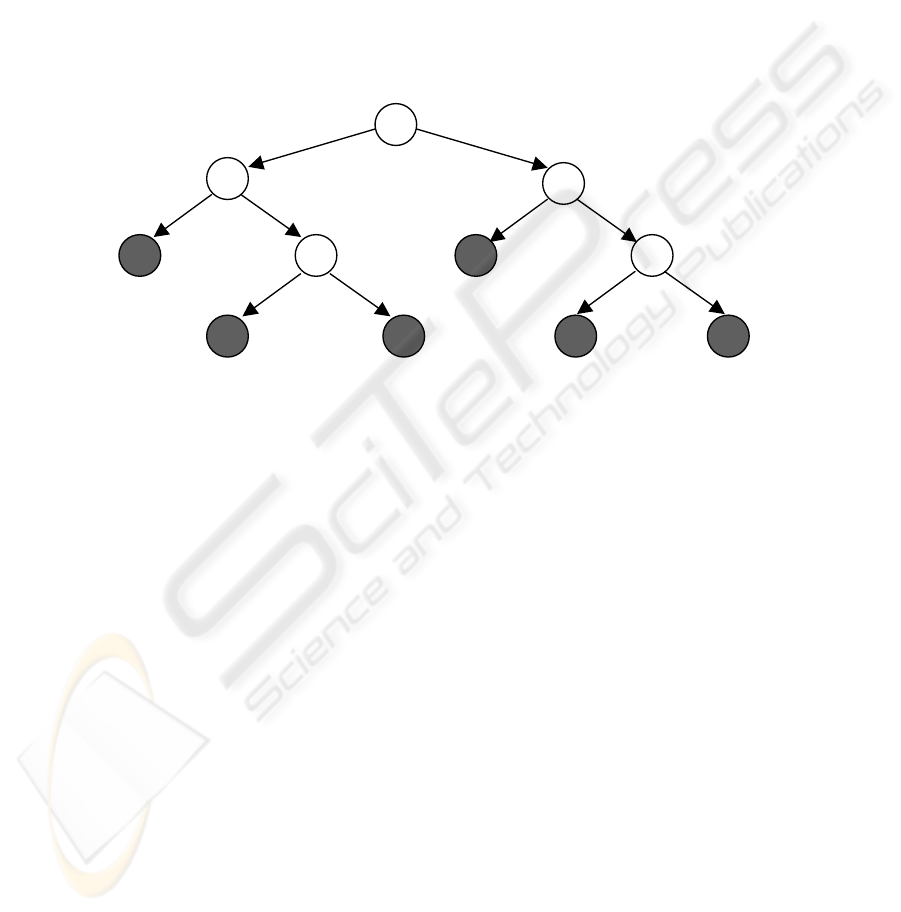
Fig. 1. A neural network tree.

Figure 1 shows an example of neural network trees. A neural network tree is a deci-

sion tree, which each non-terminal (internal) node being an expert neural network.

We can consider a neural network tree as a modular neural network [5]. To design a

neural network tree, we can use the same recursive process as that is used in conven-

tional algorithms [6]. The only thing to do is to embed some algorithm in this process

to design each expert neural network, e.g. a simple genetic algorithm into C4.5 [6]

algorithm. To simplify the problem, we have two assumptions: 1) The architecture of

all expert neural networks are the same (a multilayer perceptron with the same num-

ber of layers and the same number of neurons in each layer) that are pre-specified by

the user. 2) Each expert neural network has n branches, with n ≥ 2. First, by fixing

the architecture of all expert neural networks, we can greatly restrict the problem

space for finding an expert neural network for each node. Second, we allow multiple

branches because each expert neural network is not only a feature extractor, but also a

local decision maker. An expert neural network can extract complex features from the

given input vector, and then assign the example to one of the n groups. To design the

expert neural networks, the efficient way seems to be evolutionary algorithms, be-

cause we do not know in advance which example should be assigned to which group.

The only thing we can do is to choose one expert neural network, to optimize some

criterion. For this purpose, we can use a simple genetic algorithm containing merely

basic operations: one-point crossover and bit-by-bit mutation. The genotype of a

multilayer perceptron is the concatenation of all weight vectors (including the thre-

shold values) represented by binary numbers. The definition of the fitness is domain

dependent. The fitness can be defined as the information gain ratio that is used as the

criterion for splitting nodes. The basic idea is to partition the current training set in

such a way that the average information required to classify. For detailed discussion,

refer to [6].

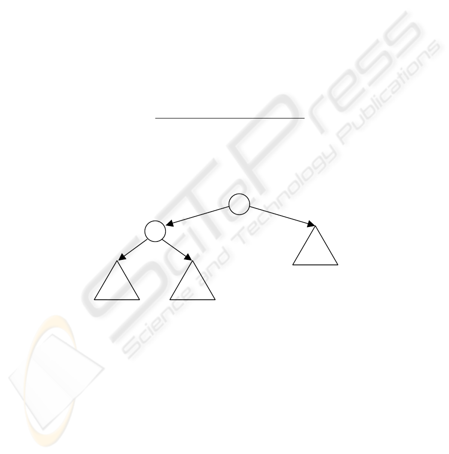
We used the top-down method [2] to design a neural network tree. In this method,

we divide the whole training set into two parts first and classify them into two catego-

ries: patterns which belong to the left-nodes, and those which belong to the right-

nodes. Figure 2 illustrates this idea. In this figure, a circle is a node, a triangle is a

sub-tree. The sub-trees are designed separately using genetic algorithm for classifying

some of the patterns in the training set. Suppose that there are n patterns in the i-th

class, n

patterns are classified to the left-nodes, and n

= n - n

patterns are classified

to the right-nodes. To evaluate a sub-tree, we provide all training patterns (in the

current training set) to the tree, assign each pattern to a proper category (left or right),

and then count the number of correct classifications. Then, the fitness can be defined

settrainingofsize

ifationmisclassifofnumber

fitness

___

1−= .

(1)

This process is repeated until the current training set contains only patterns of the

same class. Size of the whole decision tree is roughly the sum of size of all sub-trees

obtained in the recursive procedure.

sub-tree L

sub-tree R

sub-tree L

Fig. 2. Divide a tree into many sub-trees.

The neural network tree works as follows. The input is given to the root node first.

It is then assigned to the i-th child if the i-th output of the module is the maximum. If

the child is a leaf, the final result is produced locally; otherwise, repeat the same pro-

duce recursively. The most notable feature of a neural network tree is that it consists

of homogenous neural networks that can be realized using exactly the same functional

components (with different parameters), and the whole system can be constructed

hierarchically. From such neural network tree, we can easily get an autonomous mod-

ular neural network [5]. For example, if the root is a multilayer perceptron with n

outputs, it can be split into n subnets. These subnets can be used to work together

with the children. The autonomous modular neural network works like this: for a

given input task, each module tries to give an output y along with a number c. If c

the maximum, the output of the i-th module will be used as the final result. Each

module can be an autonomous modular neural network again, which is obtained from

the neural network tree by using the same procedure recursively. The basic idea is to

design small expert neural networks to extract certain features (and make local deci-

sion based on the features) first, and the overall decision can be made by the whole

decision tree.

4 Modular Neural Network

Several characteristics of modular architectures suggest that they should learn faster

than networks with complete sets of connections between adjacent layers. One such

characteristic is that modular architectures can take advantage of function decomposi-

tion. If there is a natural way to decompose a complex function into a set of simpler

functions, then a modular architecture should be able to learn the set of simpler func-

tions faster than a monolithic multilayer network. In addition to their ability to take

advantage of function decomposition, modular architectures can be designed to re-

duce the presence of conflicting training information that tends to retard learning. We

refer to conflicts in training information as crosstalk and distinguish between spatial

and temporal crosstalk. Spatial crosstalk occurs when the output units of network

provide conflicting error information to a hidden unit. This occurs when the back-

propagation algorithm is applied to a monolithic network containing a hidden unit

that projects to two or more output units.

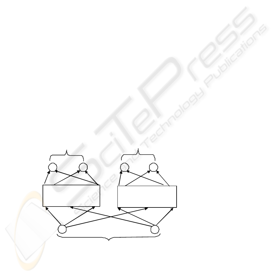
input layer of units

. . .

output layer of units

units subsistent to

module 1

units subsistent to

module k

hidden layer of units

subsistent to module l

. . .. . . . . .

. . . . . .

hidden layer of units

subsistent to module k

. . .

Fig. 3. The modular neural network architecture.

A modular architecture, which should generalize better than a monolithic network,

involves the difference between local and global generalization. Modular architec-

tures perform local generalization in the sense of the architecture that only learns

patterns from a limited region of the input space. Therefore training a modular archi-

tecture on a training pattern from one of these regions should not ideally affect the

architecture’s performance on pattern from the other regions. Modular architectures

tend to develop representations that are more easily interpreted than the representa-

tions developed by single networks. As a result of learning, the hidden units of the

system used in separate networks for the tasks contribute to the solutions of these

tasks in more understandable ways that the hidden units of the single network applied

to both tasks. In modular networks, a different set of hidden units is used to represent

information about the different tasks, see figure 3.

5 Experiments

During our experimental work, we made a very easy comparative adaptation study. In

order to test the efficiency of described algorithms, we applied them to the Fisher's

Iris data set [7] that is the bench test database from the area of machine learning. The

Fisher's Iris data set is a multivariate data set introduced by Sir Ronald Aylmer Fish-

er. The dataset consists of 150 samples from each of three species of Iris flowers (Iris

setosa, Iris virginica, and Iris versicolor). Four features were measured from each

sample; they are the length and the width of sepal and petal. Based on the combina-

tion of the four features, Fisher developed a linear discriminated model to determine

which species they are. We used 100 examples for training and the remainder for

testing.

Neural Network Tree. Expert neural networks are multilayer perceptrons of the

same size 4 - 2 - 2, where four neurons are in the input layer, two neurons are in the

hidden layer, and two neurons are in the output layer. For any given examples it is

assigned to the i-th subset, if the i-th output neuron has the largest value (when this

example is used as input). All nets are fully connected. To find such expert neural

network for each node, we adopt the genetic algorithm, which has the following

parameters: number of generation is 1000, the population size is 30, selection rate is

0.9 (e.g. 90% of individuals with low fitness values are exchanged in each

generation), crossover rate is 0.7, and mutation rate is 0.01. The number of bits per

weight is 16. The fitness is defined directly as the gain ratio. The desired fitness is

0.9. The maximum fitness is 1.0 from its definition. All individuals are sorted

according to their priority ranks, and the worst p × N individuals are simply deleted

from the population, where p is the selection rate, and N is the population size. In

each experiment, we first extract a subnet from the whole training set, and use it for

designing (training) a neural network tree. Of course, we count the number of

neurons contained in the whole tree.

Modular Neural Network. We used a three-layer feedforward neural network with

architecture is 4 - 6 - 3 (e.g. four neurons in the input layer, six neurons in the hidden

layer, and three neurons in the output layer) in our experimental work. Each module

has two neurons in a hidden layer and one output neuron. The input layer and the

hidden layer are fully interconnected. The input values from the training set were

transformed into interval <0; 1> to be use backpropagation algorithms for adaptation.

The backpropagation adaptation deals with the following parameters: learning rate is

0.3, and the moment parameter was not used.

Multilayer Neural Network. We used a fully connected three-layer feedforward

neural network with architecture is 4 - 4 - 3 (e.g. four units in the input layer, four

units in the hidden layer, and three units in the output layer) in our experimental

work, because the Fisher's Iris data set [7] is not linearly separable and therefore we

cannot use neural network without hidden units. The backpropagation adaptation

deals with the same parameters like in the previous model.

6 Conclusions

In this paper, we have studied adaptation process of neural network trees, modular

neural network and conventional neural network. Experimental results with a recogni-

tion problem show that neural network tree whose nodes are expert neural networks

is a neural network model with a comparable quality like modular neural network.

Both models have better adaptation results than conventional multilayer neural net-

work architecture but the time complexity for trained neural network trees increases

exponentially with the number of inputs, rather the size (i.e. the number of hidden

neurons) of each network. Thus it is necessary to reduce the number of inputs [3].

This is impossible for conventional neural networks because the number of inputs is

usually fixed when the problem is given.

Table 1. Table of results.

Neural network tree Modular neural network Multilayer neural network

average

error value

1.5% 1.2% 3.7%

All models solve the pattern recognition task from the Fisher's Iris data set [7] in

our experiments. The dataset consists of 150 samples from each of three species of

Iris flowers (Iris setosa, Iris virginica and Iris versicolor). Four features were meas-

ured from each sample, they are the length and the width of sepal and petal. Based on

the combination of the four features, Fisher developed a linear discriminated model to

determine which species they are. The data set was divided into two sets: the training

set contained 100 patterns and the test set 50 patterns. The error values for the train-

ing set were always near zero because perfect training was performed. Table 1 shows

a table of results. There are shown average error values for the test set over 10 runs.

Other numerical simulations give very similar results. In the future, we will study

properties of neural network trees in detail, and try to propose better evolutionary

algorithms for their designing.

References

1. Takeda, T., Zhao Q. F., and Liu, Y.: A study on on-line learning of NNTrees. In: Proc.

International Joint Conference on Neural Networks, pp. 145-152, (2003).

2. Zhao, Q. F.: Evolutionary design of neural network tree -integration of decision tree, neural

network and GA. In: Proc. IEEE Congress on Evolutionary Computation, pp. 240-244,

Seoul, (2001).

3. Mizuno, S., and Zhao, Q. F.: Neural network trees with nodes of limited inputs are good for

learning and understanding. In: Proc. 4th Asia-Pacific Conference on Simulated Evolution

And Learning, pp. 573-576, Singapore, (2002).

4. Endou, T. and Zhao, Q.F.: Generation of comprehensible decision trees through evolution

of training data. In Proc. IEEE Congress on Evolutionary Computation (CEC‘2002) Hawai,

2002.

5. Zhao, Q. F.: Modelling and evolutionary learning of modular neural networks. In: Proc.

The 6-th International symposiums on artificial life and robotics, pp.508-511, Tokyo

(2001).

6. Quinlan, J. R.: C4.5: Programs for machine learning. Morgan Kaufmann Publishers,

(1993).

7. http://en.wikipedia.org/wiki/Iris_flower_data_set (from 16/1/2009).

8. Di Fernando, A., Calebretta, R., and Parisi, D.: Evolving modular architectures for neural

networks. In French R., and Sougne, J. (eds.).Proceedings of the Sixth Neural Computation

and Psychology Workshop: Evolution, Learning and Development. Springer Verlag, Lon-

don, 2001.

9. Fausett, V. L.: Fundamental of Neural Networks, Architecture, Algorithms and Applica-

tions, Prentice Hall; US Ed edition, 1994.