
Semi-automatic Detection of Corticalis Borders in
Two-dimensional Radiographies to Improve
Pre-operative Planning
Marc Schlimbach and J¨urgen Wahrburg
Center for Sensor Systems (ZESS), Siegen University
Paul-Bonatz Street 9-11, 57076 Siegen, Germany
Abstract. This paper suggests an algorithm to detect corticalis borders in a ra-
diograph. It is robust against occurring interferences in radiographies, because it
is a global working procedure. This segmentation is part of semi-automatic as-
sistant functions, which are developed to support surgical interventions. The al-
gorithm will be introduced related to the calculation of the femoral CCD-Angle.
Further subjects of the presented proposal cover special aspects when using a
two-dimensional radiography for pre-operative planning instead of CT or MRT
scans.
1 Introduction
The work outlined in this paper is embedded in the development of the modiCAS as-
sistant system. modiCAS is the abbreviation for modular interactive computer assisted
surgery. It is a system to support the surgeon during surgical interventions. This pa-
per describes the determination of important surgical parameters which may later be
used during the intervention supported by navigation systems or a robot based assistant
system.
Radiography is the most used modality in orthopaedics and trauma surgery. The
challenge consists in extracting as many parameters as possible out of radiographies
during the planning phase to allow an optimal prearrangement of the intervention. An
additional problem is the scaling of radiographies. In contrast to the scaling of CT
or MRT scans, projection images of two-dimensional x-ray scanners do not contain
inherent scaling information.
Due to the intraoperative use of c-arms, radiographies are also generated during the
intervention. So it is possible to extract parameters to control a mechatronical assistant
system. For this task the scaling of radiographies is very important.
Thus there are several applications where the accurate and easy extraction of impor-
tant parameters for a surgical intervention is of high relevance. In order to support the
user here, we develop semi-automatic assistant functions within the modiCAS project.
A semi-automatic assistant function is a combination of automatic functions and
manual steps. All parameters which are computed automatically by an algorithm will
be transferred to a planning object. These planning objects allow the user interaction,
Schlimbach M. and Wahrburg J. (2009).
Semi-automatic Detection of Corticalis Borders in Two-dimensional Radiographies to Improve Pre-operative Planning.
In Proceedings of the 1st International Workshop on Medical Image Analysis and Description for Diagnosis Systems, pages 62-73
DOI: 10.5220/0001814500620073
Copyright
c
SciTePress
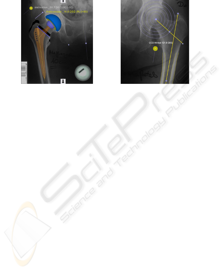
Fig.1. Screenshot of a hip replacement
planning with modiCAS-Planning.
Fig.2. Femur and neck axis to measure
the CCD-angle.
and the user has the chance to manipulate the parameter before he starts the next step
of the semi-automatic assistant function.
One advantage of such an assistant function compared to the manual creation of
planning objects is the advantage in time. Even in the case of planning standard inter-
ventions like hip replacements, time requirements play an essential part for the accept-
ability of such a planning tool.
This paper suggests a procedure to allow the fast and safe segmentation of long
bone corticalis borders in radiographies. This procedure is the base of a semi-automatic
assistant function to determine the CCD-angle of a femur bone. In a further step this as-
sistant function will make a proposal for the optimal femoral implant out of a database.
2 Problem
Hip replacement proceduresrequire the pre-operativeplanning of a pelvic and a femoral
component. For each component an appropriate size and type must be selected out of
a database. In the next step this component must be placed in the image data. Figure 1
shows a screen shot with a complete planning and three-dimensional implant models.
This planning is carried out using the software modiCAS-Planning.
The presented semi-automatic assistant function supports the surgeon during the plan-
ning of the femoral shaft component. Some patient specific parameters must be deter-
mined out of a radiograph to select a fitting shaft implant.
Figure 2 shows the femoral axis and the neck axis which are two of these param-
eters. The angle between these axes is the CCD-angle. Apart from the size the CCD-
angle is an important criterion to select the shaft implant. Implant manufactures offer
shaft implants with different CCD-angles in adaptation to the varying anatomy of dif-
ferent patients.
63
It is possible to compute the femoral axis out of the corticalis borders with a smooth-
ing function. The shown rotation center of the head is one point of the neck axis. In
addition to the CCD-angle the corticalis borders and the rotation center of the head are
other criteria which are important during the implant selection.
The proposedprocedureto determine the corticalis borders should be released within
the existing surgical tool modiCAS-Planning. The functionality will be explained at the
femoral bone. The aim is to support the user during the implant selection and position-
ing of a shaft.
3 Specific Aspects using Radiographies
If radiographies are used for planning, it will be important to take some specific aspects
in consideration.In this paper two aspects are discussed. The first aspect is the scaling of
radiographies. The second aspect is the reconstruction of three-dimensional information
out of a series of two-dimensional radiographies.
3.1 Scaling of Radiographies
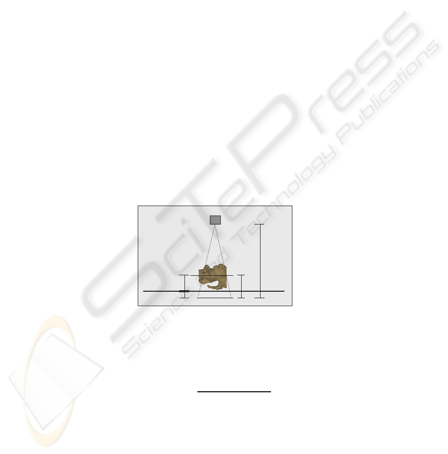
As known radiography is a projection bases technology. Depending on the arrangement
(Figure 3) of x-ray source, x-ray detector and patient the recorded image appears greater
by a certain image scaling factor (1). For measurement of length in radiographies the
scaling factor must be known, but it is a problem to determine the correct one.
Source-Detector
Plane-Detector
X-raysource
X-raydetector
Table
scalingplane
Fig.3. Assembly of an X-ray equipment for radiography.
The scaling factor (1) describes the size difference between a pixel on the detector
and the imagined region in the patient.
F
scale
=
S
SourceT oDetector
S
SourceT oP lane
(1)
In this equation S
SourceT oDetector
is the distance between the focus of the x-ray source
and the x-ray detector. The value of S
SourceT oP lane
is the distance between the focus
and a plane through the patient which is parallel to the x-ray detector. The height of this
scaling plane above the detector depends on the one hand on the use case and on the
64
other hand on the individual anatomy of the patient. These two dependences will be not
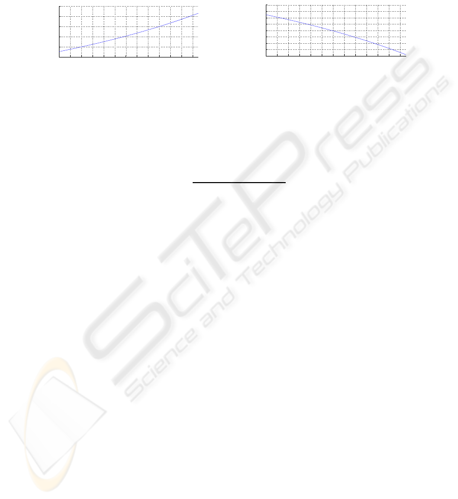
reflected, if a standard scaling factor is used. The dependency between scaling factor
and scaling plane is shown in Figure 4.
5 7 9 11 13 15 17 19 21 23 25 27 29
1
1.1
1.2
1.3
1.4
1.5
Height [cm]
1 / scaling factor
Fig.4. Scaling factor depending on the
height of the scaling plane. The distance
between focus and detector is 100 cm.
5 7 9 11 13 15 17 19 21 23 25 27 29
−20
−15
−10
−5
0
5
10
15
20
Height [cm]
Scaling error [%]
Fig.5. Percental scaling error by using a
standard scaling factor of 1:1.2 depend-
ing on the height of the scaling plane.
In equation (2) the scaling factor depends on the distance h between the x-ray detector
and the scaling plane through the patient.
F
scale
=
S
SourceT oDetector
S
SourceT oDetector
− h
(2)
Figure 5 shows the percentage error which will occur, if a standard scaling factor of
1:1.2 is used instead of the correct scaling factor. The graph illustrates the scaling error
of round about one percent for every centimetre change in altitude.
There are the following consequences relating to the selection of a cup implant.
Usually cup implants are available in size steps of 2 mm. The percentage difference
between a cup with a diameter of 56 mm and one with 58 mm is round about 3.5% for
example. So it is possible to plan a cup that differs in one or two size steps to the cup
which is needed.
It is clear that the standard scaling factor, which is often used in DICOM files,
allows no exact measurements. Another area where such standard scaling factors are
applied, are two-dimensional implant templates. These templates are used to make a
manual planning on not scaled radiographies by using a light box.
One possible solution to reduce this problem is a scaling body with a known size. This
scaling body must be placed in the radiography on the height of the required scaling
plane. At the beginning of a new planning the size of this scaling body can be measured
in the image to get the scaling factor. The accuracy of a scaling factor which is deter-
mined in that way depends on the error which is made by placing the calibration body
on the required height. If only angles like the CCD-Angle should to be measured in a
radiograph, a scaling will be not necessary.
3.2 2D-3D Reconstruction
If there is a set of radiographies available during the planning time, it will be possi-
ble to extract some three-dimensional information out of these images. Therefore it is
required, that the recording situation of each image is known.
65

There are some algorithms for this kind of three-dimensional reconstruction sug-
gested in the literature. The procedure described in [1] is qualified for pre-operative
planning. It bases on a special calibration body which must be placed in the image dur-
ing the recording time. So it is possible to reconstruct the recording situation during the
planning and pose the images in the virtual planning space.
A navigated c-arm is another possibility to get radiographies with a known record-
ing situation. With this technology the recording situation is delivered directly by the
c-arm and no complex algorithms are used by the reconstruction.
Semi-automatic assistant functions would be appropriateto generate three-dimensional
information out of such arranged radiographies during the intervention in a short time.
4 Known Procedures for Corticalis Detection
Several procedures have been developed in the last years to detect the femoral contour,
but most of these proposals were limited to the outer femoral contour. Some of the
proceduresare based on a two-dimensionalfemur model, which is registered atlas based
in the first step. In the second step a fitting procedure deforms the two-dimensional
model to the real contours in the x-ray. The active contour algorithm is one option to fit
the model. [4], [6].
Another possibility is the deformation of a three-dimensional statistical model as
described in [5]. This approach needs more than one radiograph. In addition the orien-
tation between the radiographies is required. This work makes a proposal of a procedure
that detects the inner and outer contour of a corticalis in a fast and stable way.
5 New Procedure to Detect Corticalis Borders
Radiographies often have interferences like shades, channels or local overlapping. Due
to this it is complicate to get good and save results with procedures which have a lo-
cal operation method like the path finding algorithm. Another problem which must be
solved to use a path finding algorithm is the detection of the starting points. The new
proposal of this paper has a global operation method. Due to this it has the advantage
to be more robust against local interferences.
The procedure of this proposal is divided in several steps. Within these steps some
standard methods out of the image processing are used. The general functionality is as
follows. At first as many as possible groups composed of 4 points were build. Each of
these points should be a part of the corticalis borders. The following steps process some
plausibility tests to filter out point groups that don’t completely belong to the corticalis
borders.
5.1 Compute Gradients
The first step computes the gradient in x-direction. This is done by a Sobel operator (3)
from [2]. The advantage of this operator is its small angle error. Further the gradient
image will be normalized.
66

H
S
′
x
=
3 0 − 3
10 0 −10
3 0 − 3
(3)
5.2 Quadruple Building
In this step the gradient image of the previous step will be processed line by line. If
the application requires only some interpolation points of the corticalis borders, it will
be possible to process only each n-th line of the image. The size of n depends on the
required distance between the interpolation points.
The criteria which are used to decide weather an image point belongs to the searched
contour or not are derived from the following considerations.
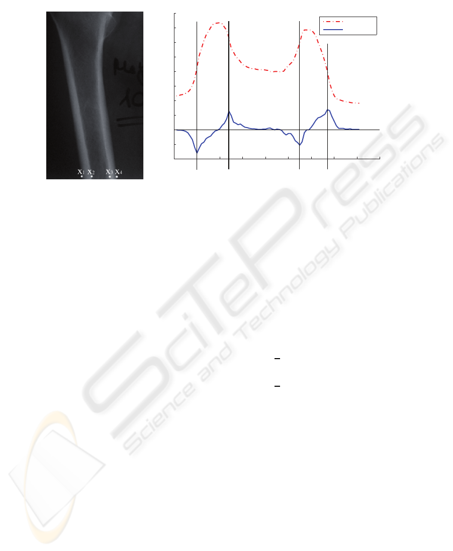
The gradient through a bone in x-direction has a typical history shown in Figure
6. The recognizable minima and maxima of the inner and outer corticalis borders are
named with x
1
· · · x
4
. Such a group of four points will be named as a quadruple in
the following text. In a quadruple x
1
and x
3
represents minima, x
2
and x
4
represents
maxima. A further condition for a quadruple is that the Points x
1
· · · x
4
are in rising
x-direction. There are some advantages caused by the combination of four points to a
quadruple:
– It is possible to define requirements, which must be fulfilled by each quadruple.
– It is possible to compute the center point of each quadruple. The center points of
one femur must be up to a line approximately.
– In the end it will be sure that there is the same number of points on both femoral
sides. Due to this it will be simplified to compute the center axis of the bone with a
linear smoothing function.
The algorithm creates two lists, to identify all possible quadruples of the current
image row. The first list stores all positions of the row where the gradient reaches a local
maximum. The second list stores all positions of local minima. Thereto the algorithm
runs through the current image row and detects minima and maxima in an alternating
way. A new extrema will be found, if the magnitude decreases in the following at least
80% or brakes through the zero line.
After detecting all extreme positions of the current image row only the extreme
positions with the biggest magnitude of the gradient will be used furthermore, to sup-
press noise and other interferences. A pelvic overview with two femora contains 4 max-
ima and 4 minima which are interesting. By disturbance or other objects like radiation
protectors there could be other vertical edges which produce extreme positions in the
horizontal gradient. These extrema could have a higher magnitude than the searched ex-
treme positions. Based on the experience of our tests a maximum number of 15 minima
and 15 maxima are adequate to be sure that the searched extreme positions are included.
After this the algorithm builds all possible quadruples out of the maximal 30 local
axtrema. Each of these combinations will be tested with several criteria. If a quadruple
passes all tests, it will be saved as a candidate of the current image row for further
processing steps.
67
0 10 20 30 40 50 60 70 80 90
−40
−20
0
20
40
60
80
100
120
140
160
x−position
gradient and gray value
gray value
gradient
X1 X4X3X2
Fig.6. Gray value and gradient in x-direction through a femur with the extreme positions
x
1
· · · x
4
.
These tests analyze several characteristics of the gradient at the positions x
1
· · · x
4
and can be divided in two groups. The first group is responsible for the magnitude of
the gradient in the extreme positions. The second group checks the geometrical charac-
teristics.
The following rules represent the conditions of the gradients magnitude.
|2 · grad(x
1
)| > |grad(x
2
)| (4)
|2 · grad(x
4
)| > |grad(x
3
)| (5)
||grad(x
1
)| − |grad(x
4
)|| <
1
2
(6)
||grad(x
2
)| − |grad(x
3
)|| <
1
2
(7)
The inequality (4) is based on the observation that the minimum at position x
1
is usually
bigger than the maximum at position x
2
. The rule (5) follows analogous to that for the
positions x
3
and x
4
. The rules (6) and (7) are the results of the fact that the magnitude
of the extremums at x
1
and x
4
respectively x
2
and x
3
are round about the same size.
The following substitutions are introduced for better expression of the geometrical
rules.
w
CR
= x
2
− x
1
(8)
w
CL
= x
4
− x
3
(9)
d
1
= x
4
− x
1
(10)
d
2
= x
3
− x
2
(11)
68
w
CL
and w
CR
are the latitudes of the left respectively right corticalis. The outer and
inner diameter of the bone is described with d
1
and d
2
.
The latitudes of the left and right corticalis usually do not vary more than a factor
of two. This is the reason of inequality (12). The proportions between the left and right
corticalis on the on hand and the inner and outer diameter on the other hand are for-
mulated with the rules (13, 14, 15, 16). The acceptable ratio between inner and outer
diameter is formulated with rule (17). The factors which are used in these rules are se-
lected in a way that no quadruple of the test data will fail a test, if it is completely up to
the femoral corticalis borders.
1
2
w
CR
< w
CL
< 2 · w
CR
(12)
0.5 · w
CL
< d
2
< 5 · w
CL
(13)
0.5 · w
CR
< d
2
< 5 · w
CR
(14)
8 · w
CL
> d
1
(15)
8 · w
CR
> d
1
(16)
4.2 · d
2
> d
1
> 1.2 · d
2
(17)
5.3 Localise the Femora
In this step the algorithm detects the number of bones and the detected quadruples will
be attached to the different bones. In the case of femur detection there can be an image
with one or two femora.
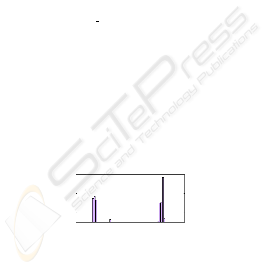
Therefore the x-axis will be divided into three parts of equal length, and the centre
point as the arithmetic average of the four points will be computed for each quadruple.
On basis of the centre point position the algorithm allocates each quadruple to one
of the three segments. When all quadruples are attached to a segment the number of
quadruples per segment can be compared (Figure 7).
0
10
20
30
40
50
x−position
number of quadruples
Fig.7. Distribution of the centre points over the x-axis in the case of a pelvic overview.
If the left and the right segment have more quadruples than the inner segment, the
image is a pelvic overview with two femora. In this case the quadruples which are
69

attached to the inner segment will be deleted and the quadruple attached to the outer
segments will be attached to two femoral objects. In the other case only one femur is
visible in the image and the algorithm use the quadruples of the inner segment to build
one femoral object
5.4 Filtering with the Hough Transformation
This step will be passing through for each detected femur. It computes a first estimation
of the center axis of the quadruples which are attached to a femur.
At this time the algorithm assumes that most of the points which are attached to a
femur are up to the corticalis contour. Due to this there will be a clearly straight, if the
center points of each quadruple that is attached to a femur will be painted in an image.
Although there may be some quadruples with center points more or less far away from
this axis. This points can be called as noise.
For estimation of the center axis a procedure is needed that is robust against these
outliers. The Hough transformation for line detection is one candidate. The result of
the Hough transformation is only influenced by the points which are part of the line.
All other points have no influence to the result as long as there is no accumulator filed
with more points than the accumulator field of the searched straight. Alternatively we
have made some trails with a smoothing function. But at this processing time there can
be too much center points far away from the bone axis. These points would have a big
influence to the results of such a smoothing function particularly combined with short
bone segments. In this case there will be only a low number of image rows and the
influence of such outlier increases.
However, the Hough transformation has a further big advantage, because it is very
simple to shrink the allowed range of angles. If images with perpendicular aligned bones
like femora are processed, the asked straight will be as well more or less perpendicular
aligned.
The distance between the center point and the estimated bone axis is the criterion
for filtering in this step. To define a limit for this distance the standard derivation of the
distance of all center points will be computed. Afterwards all quadruples with a greater
distance between their center point and the estimated axis than the calculated standard
derivation will be filtered out.
5.5 Final Filtering
The last step is the filtering procedure with a smoothing function. Thereto the algorithm
computes a best-fit line with a smoothing function based on the method of smallest
square deviation.
If there are more than one quadruple per image row and femur, the quadruple with
the closest center point will be selected. All other quadruples will be filtered out and a
recalculation of the best-fit line starts.
The final best-fit line is the center axis of the bone.
70

6 Realization within the Modicas Software Framework
The suggested procedure was realized as plug-in of the surgical planning software
modiCAS-Planning which is a part of the modiCAS-Project. This project realizes the
complete chain of a surgical intervention.
Therefore it is possible to create a planning based on two- or three-dimensional
modalities. Afterwards the surgeon can be supported during the intervention by a mecha-
tronical assistant system.
The planning software is designed as a framework. Further it has a plug-in interface
to allow simple appending of new functions to the system. Additional the software has
an own scripting language to bind the operations of a planning or an intervention in
a workflow. The advantage of this workflow concept is the easy and fast method of
interaction. The user will be guided step by step and there is no need to select the next
function manually. To support the new functions of the plug-ins in a workflow, it is
although possible to extend the scripting language via plug-ins.
The plug-in which was developedto demonstrate the procedure is able to create line
planning-objects for the femoral axis and contour planning-objects for the corticalis
borders, which can be used for further planning steps.
A second plug-in was realized for semi-automatic scaling of radiographies. This
plug-in detects a round calibration body with the procedure suggested in [3]. The sug-
gested algorithm bases on the detection of vectors with opposite directions. If a calibra-
tion body is found, the plug-in creates a circle planning object which will be modified
by the user, if there is any need. After confirmation by the user the image will be scaled
to the correct size.
7 Discussion
The procedure was validated with twenty radiographies from five different X-ray equip-
ments for radiography. These images contain 29 femora which should be detected. The
results have been compared to manual created femoral axis.
It is enough to get some base points of the corticalis borders to compute the femur
axis. The pixel distance between these points depends on the image resolution and the
expected size of the bone. During this validation, the algorithm worked on each 10th
image row. The reason for this is the decreasing computing time which is important in
a semi-automatic assistant function to produce no time of waiting for the user.
It was possible to detect whether the image was a pelvic overview with two femora
or a single sided radiography. There was only one image with a detected quadruple
which doesn’t belong to a femur. Figure 8 shows the result of one of the images.
In the upper part of the femur, where the corticalis becomes smaller, not all quadruples
were found, but this makes no big difference concerning the calculation of the femoral
axis.
The detection of the outer corticalis contour was robust. On the inner side there are
5 of 29 femora with inaccuracies in one or two of the detected quadruples. In all of
these cases an inner contour point is moved too much in the direction of the femoral
center axis (Figure 9). Due to the low number of faulty points this has no consequence
71
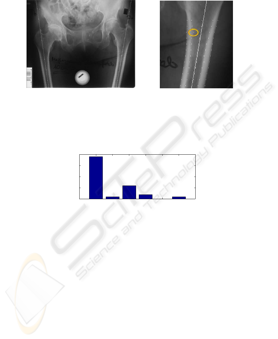
Fig.8. Detected quadruples and femur
axis within the original radiography.
Fig.9. Faulty pixel of the inner femoral
corticalis border.
to the detection of the femoral axis. It should be able to resolve this problem by a post
processing of the contour points.
0 1 2 3 4 5
0
5
10
15
20
error in degree
quantity
Fig.10. Results of the validation. 28 of 29 femora were detected in 20 radiographies.
Figure 10 shows the differences between the detected femoral axes compared to the
manual created axes. In 19 of 28 cases there were no error. One femur could not be
found.
Also radiographies of patients who already had one or two implants were tested. In
these images it was possible to detect the corticalis only below the implant.
The presented algorithm needs a vertical aligned long bone. In the tested images the
femora were rotated 13
◦
at maximum. In this rage of rotation no degeneration of the
results could be observed. If it is known that the long bone is horizontal aligned, it will
be possible to rotate the image or to use image cols instead of image rows during the
computation.
Due to these results the suggested procedure to detect long bone corticalis borders
is stable and accurate enough to use it in combination with the semi-automatic assistant
function described in this paper. Similarly the computing time round about 4 seconds
on a standard computer is short enough.
72

Table 1. Differences between manual and automatic detected femoral axes.
Results
minimal derivation 0
◦
maximal derivation 5
◦
standard derivation 1,53
◦
not founded femora 1
In the next time we will validate the procedure with an expanded amount of images.
Additionally we plan to test the algorithm with other types of bones.
8 Conclusions
This contribution explained a procedure to detect the corticalis borders of a long bone.
The procedure was classified by describing the use cases and alternative procedures.
The stable and accurate detection of the femoral axis and the femoral corticalis
borders and their use in a semi-automatic assistant function was the reason to develop
the presented procedure.
The suggested procedure was realized as a plug-in for the surgical planning tool
modiCAS-Planning. First steps of the validation were auspicious.
References
1. Groß, I.: Entwicklung eines Softwaresystems zur universellen Planung chirurgischer Ein-
griffe an 2D- und 3D- Bildmodalit¨aten. Shaker-Verlag, Aachen (2004)
2. J¨ahne, B.: Digital Image Processing: Concepts, Alogorithms and Scientific Applications. 6th
revised and extended edition. Springer-Verlag, Berlin Heidelberg New York (2002)
3. Rad A. A., Faez K., Qaragozlou N.: Fast Circle Detection Using Gradient Pair Vectors. Lec-
ture Notes in Computer Science. Springer-Verlag, Berlin Heidelberg New York (2003) 879-
887
4. Chen Y., Ee X., Leow W. K., Howe T. S.: Automatic Extraction of Femur Contours from
Hip X-Ray Images. Lecture Notes in Computer Science. Springer-Verlag, Berlin Heidelberg
New York (2005) 200-209
5. Dong X., Zheng G., Ballester M.A.G.: Automatic Extraction Of Femur Contours From Cal-
ibrated X-Ray Images: A Bayesian Inference Approach. Applications of Computer Vision,
IEEE Workshop. I. C. Society, Hrsg. (2007)
6. Kiattisin S., Chamnonghtai K.: Noninvasive Femur Bone Volume Estimation Based on X-
Ray Attenuation of a Single Radiographic Image and Medical Knowledge. IEICE Transac-
tions on Information and Systems. (2008) 1176-1184
73
