EIGENVECTOR ANALYSIS FOR OPTIMAL FILTERING

UNDER DIFFERENT LIGHT SOURCES

Juha Lehtonen, Jussi Parkkinen

Department of Computer Science and Statistics, University of Joensuu, P.O. Box 111, FI-80101 Joensuu, Finland

Timo Jaaskelainen

Department of Physics and Mathematics, University of Joensuu, P.O. Box 111, FI-80101 Joensuu, Finland

Alexei Kamshilin

Department of Physics, University of Kuopio, P.O. Box 1627, FI-70211 Kuopio, Finland

Keywords: Color spectrum, Eigenvector, Filtering, Illuminant, Sampling interval.

Abstract: Eigenvectors from Standard Object Colour Spectra (SOCS) set were used with several other spectra sets to

find the optimal sampling intervals for optimal number of eigenvectors. The sampling intervals were

calculated for each eigenvector separately. The analysis was applied not only for different sets of reflectance

spectra, but also for spectra sets under different real light sources and standard illuminations. It is shown

that 20 nm sampling interval for eigenvectors from SOCS set can be used for reflectance data and data

under such light sources which spectrum is smooth. However, data under peaky real fluorescent light

sources and standard F-illuminant require accurate 5 nm or even narrower sampling interval for the first few

eigenvectors, but can be wider with some of the others. These eigenvectors from SOCS set are shown to be

applicable for the other data sets. The results give guidelines for the required accuracy of eigenvectors under

different light sources that can be considered e.g. in eigenvector-based filter design.

1 INTRODUCTION

Color is usually represented with three components,

such as with RGB color coordinate system. In many

cases, this is not enough. Trichromatic

representations of color are depended on the used

device and illumination, and those are affected by

metameric issues (Morovic, 2002). These problems

can be avoided with accurate spectral representation

of color. The use of spectral color is becoming more

and more popular. Spectra are needed for example in

telemedicine (Nishibori, 2002), e-commerce, digital

art museums (Martinez et al., 2002), art restoration,

quality control (Hyvärinen et al., 1999) etc.

However, accurate spectral color measurement

devices are expensive and measurement may be

difficult in a noisy environment. Accurate non-

compressed spectral data require also a lot of

memory, which will cause problems in using, storing

and transferring tasks (Hauta-Kasari et al., 2006).

Spectral dimensionality has been widely studied.

This consists of finding the required sampling

interval of color spectra (Buchsbaum & Gottschalk,

1984; Maloney, 1986; Bonnardel & Maloney, 2000;

Lehtonen et al., 2006), and transforming the spectra

to another lower dimensional space (Parkkinen et al.,

1989; Hyvärinen et al., 2001; Schettini, 1994; Early

& Nadal, 2004). One widely used method is

Principal Component Analysis (PCA) (Parkkinen et

al., 1989), where the data dimensionality is reduced

with the eigenvectors of the data. Several

applications based on PCA, such as non-negative

filters for imaging have been developed (Piché,

2002). By Hauta-Kasari et al., (1998), the

eigenvector-based non-negative filters make it

possible to produce the inner-product set in

hardware level. From the measured data, accurate

spectral information can be computed.

However, to the authors’ knowledge, optimal

number of eigenvectors under different illuminants

Lehtonen J., Parkkinen J., Jaaskelainen T. and Kamshilin A. (2009).

EIGENVECTOR ANALYSIS FOR OPTIMAL FILTERING UNDER DIFFERENT LIGHT SOURCES.

In Proceedings of the Fourth International Conference on Computer Vision Theory and Applications, pages 95-100

DOI: 10.5220/0001798700950100

 SciTePress

combined with the required spectral accuracy of the

eigenvectors has not been studied. Here we will

create such sets of eigenvectors under different light

sources that can be used for several other color data

sets. This includes also a study of required spectral

accuracy of eigenvectors. The results can be used

e.g. in filter design to create optimal number of non-

negative color filters for different illuminants, which

can be used generally for accurate color

measurements (Piché, 2002; Hauta-Kasari et al.,

1998).

2 THEORY

A widely used method for reducing the dimensions

of color spectra is Principal Component Analysis

(PCA) (Parkkinen et al., 1989). Let C be a

correlation matrix

∑

(1)

Here S

is ith spectrum of a spectra set S and N is the

number of spectra. The h first eigenvectors of the

spectra set ordered by the largest eigenvalues can be

calculated. The inner-product set P is then formed

with equation

()

,,...,,

τττ

(2)

where

()

,...,,

and T denotes the eigenvectors

and matrix transpose, respectively. The data can be

reconstructed back to spectra with the linear

combination of

()

,...,,

and inner-product set

If spectra data set is well defined, one might use

the eigenvectors calculated from it to reduce the

dimensionality of any other spectra set. In this study,

we try to use the eigenvectors of a data set with

different other data sets and optimize the sampling

intervals of the eigenvectors. Each eigenvector was

sampled to several sampling intervals

straightforward and then interpolated back with

Lagrange interpolation used by Fairman (1985)

before reconstruction of spectra. Such number of

eigenvectors and sampling intervals were chosen

that the reconstructed spectra have good quality. For

this, several quality and error measurements were

done defined in chapter 4. This analysis was studied

with the reflectance spectra and also with spectra

under different real light sources and standard

illuminants. However, since the eigenvectors are

sampled and interpolated, those are not orthogonal

after conversion, and calculating with PCA is not

straightforward. A pseudoinverse matrix is required

to fix the orthogonality, and the reproduction can be

calculated with

() ()

rrr

ττττ

−

⎥

⎦

⎤

⎢

⎣

⎡

(3)

where

is the sampled and interpolated

eigenvectors

),,...,,(

τττ

and S

is the

reconstructed spectra set. In this study, a term

eigenvector index is used to denote the eigenvector

index number 1...h, where the eigenvectors are

ordered in descending order by the eigenvalues.

3 DATA SETS

Ten different spectra sets (University of Joensuu,

2008; Japanese Standards Association, 1998;

Kohonen et al., 2006; Funt & Lewis, 2000;

Farnsworth, 1957; Jaaskelainen et al., 1994;

Pantone, 2008) were used, listed in Table 1. The

spectra originally measured with wider sampling

interval than 1 nm were interpolated with Lagrange

method shown by Fairman (1985) to 1 nm data and

treated as original data. According to Lehtonen et al.

(2006) and Sándor et al. (2005) this can be done,

since interpolated reflectance spectra are very near

to spectra measured with 1 nm. Spectral values

outside 400...700 nm range were eliminated.

Table 1: Data sets.

Data set Nr.

spectra

Original

wavelength

area [nm]

Original

sampling

[nm]

Dupont

120 400...700 4

FM100

85 400...700 5

Wood

1,056 390...850 5

Lumber 272 380...2700 1

Munsell Glossy

1,600 380...780 1

Munsell Matte

1,269 280...800 1

Object Spectral Reflect-

ance Database (OSRD)

170 400...700 4

Pantone

922 380...780 1

Printed Colors 2,240 380...780 1

Standard Object Colour

Spectra (SOCS)

49,392 400...700 5, 10

Funt & Lewis, 2000.

Farnsworth, 1957.

Jaaskelainen et al.,

1994.

University of Joensuu, 2008.

Pantone, 2008.

Japanese

Standards Association, 1998.

At first, eigenvectors from different data sets

were tried to be used separately for other data sets.

According to tests, suitable eigenvectors can be

calculated from both Munsell sets (University of

Joensuu, 2008), from Pantone set (Pantone, 2008)

and from Standard Object Colour Spectra (SOCS)

VISAPP 2009 - International Conference on Computer Vision Theory and Applications

set (Japanese Standards Association, 1998). The

spectra of the Munsell sets and Pantone set vary a

lot. For example Munsell set describes the colors of

CIE L*a*b* coordination well, and therefore the

eigenvectors are formed for the whole coordination.

However, both Munsell sets and also Pantone set

had problems with Wood data set (Jaaskelainen et

al., 1994), requiring near 20 eigenvectors for good

result, but this problem was not an issue in any set

with eigenvectors of SOCS set. SOCS data set

includes 49,392 spectra from photographic

materials, printed colors, paints, textiles, human

skin, flowers and leaves. This is a wide collection of

color spectra and therefore, the eigenvectors of this

set can represent several types of data well.

The sampled and interpolated eigenvectors from

SOCS data set were calculated. These eigenvectors

were used as a base for calculating the inner-

products of other spectra sets and for reconstruction.

The required number of eigenvectors and the needed

sampling interval of eigenvectors were found with

calculating the quality of reconstructed spectra. The

number of eigenvectors was chosen as the smallest

possible. This procedure was also experimented with

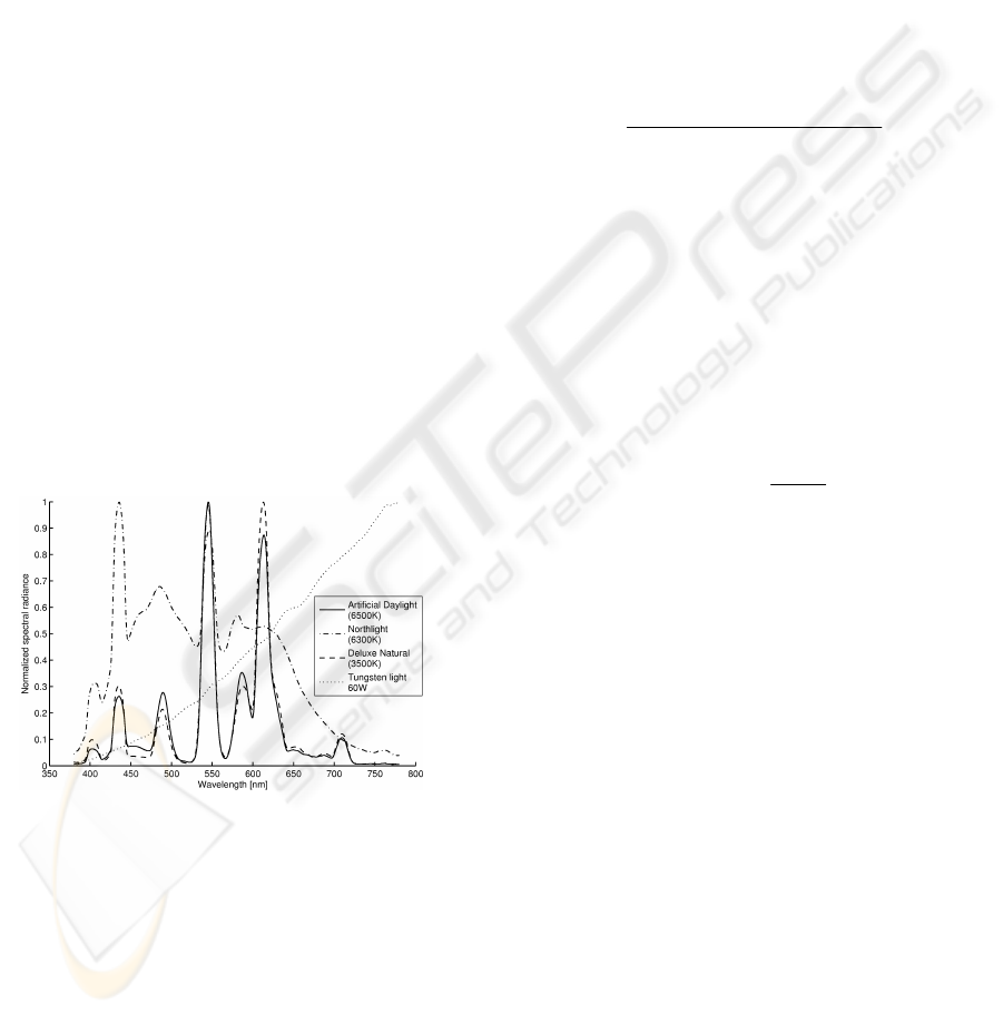
the reflectance data, data under four different real

light sources and five standard illuminants A, D65,

F2, F8 and F11. Spectra of the real light sources are

shown in Figure 1. In these cases, also the SOCS

data was converted under the light source or

illuminant before PCA calculations.

Figure 1: Spectra of the real light sources.

4 QUALITY AND ERROR

MEASURES

Two quality measures and one error measure were

used to define the quality of reconstructed spectra.

The error measure is ΔE, which measures the visual

color difference in CIE L*a*b* color coordination as

()

,***

2/1

222

baLE Δ+Δ+Δ=Δ

(4)

where ΔL*, Δa* and Δb* are the component

differences between the original and reconstructed

color values in CIE L*a*b* color space. According

to Ohta and Robertson (2005), ΔE = ~1.0 is usually

discriminable. Parkkinen et al. (1989) use color limit

of average ΔE < 0.5. Equal-energy spectrum was

used as illuminant with calculating the tristimulus

values.

Goodness-of-Fit Coefficient (GFC) (Hernández-

Andrés et al., 2001) is a correlation based quality

measure between two spectra, measuring the

similarity of two spectra. It is defined as

() ()

2/1

⎥

⎦

⎤

⎢

⎣

⎡

⎥

⎦

⎤

⎢

⎣

⎡

∑∑

∑

GFC

(5)

where n is number of channels in spectrum. Terms

s and

s are the wavelength channel values of

original and reconstructed spectra, respectively.

According to Hernándes-Andrés et al. (2001), good

limit for this quality measure is 0.999 and accurate

limit 0.995.

Peak Signal-to-Noise Ratio PSNR is widely used

quality measure in image compression, defined as

log10

MSE

PSNR

(6)

where ε

MSE

is Mean Square Error and s

is the

theoretical maximum of a channel value in

spectrum.

Based on Parkkinen et al. (1989), Ohta &

Robertson (2005) and Hernandéz-Andrés et al.

(2001), the quality and error limits were chosen as

average ΔE < 0.5, average GFC > 0.999 and average

PSNR > 40 dB. To obtain accurate results, all of

these limits must be satisfied in spectra

reconstruction. Also, when selecting a suitable

number of eigenvectors and sampling interval, it is

required that all narrower sampling intervals and

higher number of PCA components must satisfy

with the limits.

The quality and error measures and the selected

limits were compared with each other with the data

sets under Artificial Daylight source, illuminant F11

and illuminant D65. With each light source, the GFC

limit 0.999 and PSNR limit 40 dB correspond well

with each other, and both accept and reject same

sampling intervals. Similar result is found with ΔE

compared to GFC or PSNR for the data under

Artificial Daylight source. However, the ΔE limit is

EIGENVECTOR ANALYSIS FOR OPTIMAL FILTERING UNDER DIFFERENT LIGHT SOURCES

more unforgiving with data under F11 illuminant,

accepting 1...4 nm sampling intervals, whereas GFC

and PSNR accept only 1...2 nm sampling intervals.

Also, ΔE error does not always correspond with the

sampling interval. With some cases the average

visual error is smaller but the average spectral error

is higher with wide sampling interval than with

narrow sampling interval. Some small variations can

also be found with the quality measures, e.g. with

F11 illuminant GFC and PSNR values are better

with 5 nm sampling interval than 4 nm interval. For

these reasons, also all more accurate sampling

intervals than the selected one must satisfy with the

limits.

5 PARAMETER SELECTIONS

The results of the required number of PCA

components and sampling intervals of different

eigenvectors with different reflectance data sets and

data sets under Artificial Daylight source are shown

in Table 2. The eigenvectors of SOCS data is used.

For all reflectance data sets, 20 nm interval is

enough for the eigenvectors. The required number of

eigenvectors varies between 6...11, depending on the

variety of colors in data set and data set difference

from SOCS set. However, majority of the data sets

can be represented with eight eigenvectors. For data

under Artificial Daylight source, 4...6 nm interval is

needed for the first eigenvector, but can be wider

with most of the data sets with higher index

eigenvectors. Also, 4...8 eigenvectors are required

depending on the data set.

The overall results of the reflectance data sets

and data sets under different light sources are shown

in Table 3. Here, the total averages of different

quality and error measures were used, weighted

equally between different sets. With reflectance data

and data under smooth light sources the required

sampling interval for SOCS eigenvectors is 20 nm.

In average for all data sets, ten PCA components are

required with the reflectance data and data under

D65 illuminant. Eight PCA components are enough

for data under illuminant A and Tungsten light

source. The required sampling interval for the first

few eigenvectors of SOCS are 4...5 nm with data

sets under real fluorescent light sources, but interval

can be wider for higher index eigenvectors.

Depending on the light source, 5...8 PCA

components are required. For data under F-

illuminants, 1...3 nm interval is needed, but with F2

and F11, the interval can be wider for higher index

eigenvectors. In average for all data sets, 5...10 PCA

components are required depending on the light

source. It was also found that 0...2 less eigenvectors

from SOCS set are enough for the use with SOCS

spectra set alone, compared to use with other data

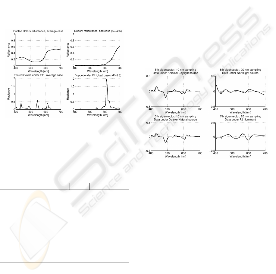
sets. Some average and bad examples of spectra

reconstruction are shown in Figure 2 when the

eigenvectors of SOCS data with sampling intervals

shown in Table 3 are used.

Table 2: Required sampling intervals of eigenvectors of

SOCS data when used with different data sets.

Reflectance Eigenvector index

data set 1 2 3 4 5 6 7 8 9 10 11

Dupont 20 20 20 20 20 20 20 20 20 - -

FM100 20 20 20 20 20 20 20 20 - - -

Forest 20 20 20 20 20 20 20 20 20 20 20

Lumber 20 20 20 20 20 20 - - - - -

Munsell G. 20 20 20 20 20 20 20 20 - - -

Munsell M. 20 20 20 20 20 20 20 20 - - -

OSRD 20 20 20 20 20 20 20 20 20 20 -

Pantone 20 20 20 20 20 20 20 20 - - -

Printed Col. 20 20 20 20 20 20 - - - - -

SOCS 20 20 20 20 20 20 20 20 - - -

Data under Eigenvector index

Artif. Dayl. 1 2 3 4 5 6 7 8

Dupont 5 4 5 11 9 11 20 10

FM100 4 7 6 11 15 - - -

Forest 5 9 9 20 13 10 8 -

Lumber 6 9 8 6 - - - -

Munsell G. 5 7 6 5 15 - - -

Munsell M. 5 7 5 11 15 - - -

OSRD 5 5 5 15 6 13 10 20

Pantone 4 7 6 9 11 14 - -

Printed Col. 5 5 9 13 14 - - -

SOCS 5 7 9 10 11 - - -

Table 3: Required average sampling intervals of

eigenvectors of SOCS data when used with all data sets

and under different light sources.

All data sets Eigenvector index

Light source 1 2 3 4 5 6 7 8 9 10

Reflectance 20 20 20 20 20 20 20 20 20 20

Artif. Daylight 5 7 5 5 10 - - - - -

orthlight 5 12 12 13 8 6 8 20 - -

Deluxe Natural 4 4 5 9 15 - - - - -

Tungsten lamp 20 20 20 20 20 20 20 20 - -

A 20 20 20 20 20 20 20 20 - -

D65 20 20 20 20 20 20 20 20 20 20

F2 1 3 5 9 13 6 20 - - -

F8 2 1 3 3 1 2 3 1 3 -

F11 2 6 3 7 6 3 7 7 - -

The spectra from each group and each light

source were divided in four groups based on the

resulted average quality and error calculations. The

average relative numbers of spectra in different error

groups for different light sources are shown in Table

4, when quality and error measures are weighted

VISAPP 2009 - International Conference on Computer Vision Theory and Applications

equally between the test sets. SOCS data was not

included in the test sets, it was only used to form the

eigenvectors. In general, over 90% of the spectra

sets are located in highest quality groups a) and b).

Only exceptions are found with Artificial Daylight

source and F11 illuminant, where the relative

number is 80%. Only about 1% of the spectra give

high error, see group d). A small exception is found

with F11 illuminant, where the number of bad

spectra is 3.8%. However, most of these spectra are

selected as bad only because PSNR values very near

30 dB is achieved, but not quite. If this quality limit

was changed to PSNR = 28 dB, the relative number

of bad spectra would be 1.6%.

Figure 2: Some average and bad examples of spectrum

reconstruction. Original spectrum is shown as solid line

and reconstructed one as dashed line.

Table 4: Relative number of spectra distributed with

quality and error measures when eigenvectors of SOCS

data with sampling interval listed in Table 3 is used.

All data sets,

not SOCS

Light source a) b) c) d)

Reflectance 83.7% 14.8% 1.5% 0.0%

Artificial Daylight 40.1% 42.8% 15.4% 1.7%

orthlight 57.4% 34.9% 6.8% 0.9%

Deluxe Natural 56.5% 35.7% 6.7% 1.2%

Tungsten lamp 68.9% 20.9% 9.0% 1.2%

A 74.3% 21.5% 3.8% 0.4%

D65 64.4% 33.8% 1.8% 0.0%

F2 56.4% 34.1% 8.3% 1.2%

F8 62.8% 26.4% 9.5% 1.3%

F11 30.5% 47.7% 18.0% 3.8%

Average 59.5% 31.3% 8.1% 1.2%

a) (ΔE < 0.5) AND (GFC > 0.999) AND (PSNR > 40dB)

b) (0.5 ≤

ΔE < 1.0) AND (0.995 < GFC ≤ 0.999) AND

(34dB < PSNR ≤ 40dB)

c) (1.0 ≤

ΔE < 3.0) OR (0.990 < GFC ≤ 0.995) OR

(30dB < PSNR ≤ 34dB)

d) (

ΔE ≥ 3.0) OR (GFC ≤ 0.990) OR (PSNR ≤ 30dB)

6 CONCLUSIONS

For reflectance data and data under those light

sources, which spectrum is smooth, the eigenvectors

are also smooth, and wide 20 nm sampling interval

is enough. For data under real fluorescent light

sources, the peaky dominating shape caused by the

light source is located in the eigenvectors, and the

required sampling interval is accurate in lower

indexes, near 5 nm, but can be a bit wider with some

higher indexes, near 10 nm. F-illuminants require

more accurate sampling interval compared to real

fluorescent light sources, between 1...7 nm

depending on the eigenvector index. Since the

higher index inner-products do not contain much

overall information, the corresponding eigenvectors

can have some more errors than lower index

eigenvectors. Few examples of errorous

eigenvectors are shown in Figure 3.

Figure 3: Some bad examples of eigenvectors with wide

sampling. Original eigenvector is shown as solid line and

reconstructed one as dashed line.

The data set under a light source, which

spectrum is peaky, require also few less PCA

components compared to reflectance data or data

under a smooth light source. The aggressive shape of

peaky light source limits the spectra more similar to

each other and therefore less PCA components are

required.

The results show also that eigenvectors defined

from large variety of data, such as from SOCS data

set, work very well generally with other data sets.

The required sampling interval of eigenvectors

depends on the eigenvector index and the light

source. All data sets under a light source give similar

sampling intervals, but the required number of

eigenvectors is different with different data sets and

light sources. However, a general required number

of eigenvectors was found for different light sources

EIGENVECTOR ANALYSIS FOR OPTIMAL FILTERING UNDER DIFFERENT LIGHT SOURCES

separately, which can be used to generate low errors.

The results can be useful in applications based on

eigenvectors, such as in designing optimal non-

negative filters for different light sources.

REFERENCES

Bonnardel V., and Maloney, L., 2000. Daylight,

biochrome surfaces and human chromatic response in

the Fourier domain, J. Opt. Soc. Am. A 17(4), 677–

686.

Buchsbaum, G., and Gottschalk, A., 1984. Chromacity

coordinates of frequency-limited functions, J. Opt.

Soc. Am. A 1(8), 885–887.

Early, E., and Nadal, M., 2004. Uncertainty analysis for

reflectance colorimetry, Color Res. Appl. 29(3), 205–

216.

Fairman, H., 1985. The calculation of weight factors for

tristimulus integration, Color Res. Appl. 10(4), 199–

203.

Farnsworth, D., 1957. The Farnsworth-Munsell 100-Hue

Test, Munsell Color Company. Baltimore, MD,

revised ed.

Funt, B., and Lewis, B., 2000. Diagonal versus affine

transformations for color correction, J. Opt. Soc. Am.

A 17(11), 2108-2112.

Hauta-Kasari, M., Lehtonen, J., Parkkinen, J., and

Jaaskelainen, T., 2006. Image Format for Spectral

Image Browsing, J. Imag. Sci. Tech. 50(6), 572-582.

Hauta-Kasari, M., Wang, W., Toyooka, S., Parkkinen, J.,

and Lenz, R., 1998. Unsupervised Filtering of Munsell

Spectra, Proc. of the Third Asian Conference on

Computer Vision, Vol. I, Hong Kong, 248-255.

Hernández-Andrés, J., Romero, J., and Lee Jr., R., 2001.

Colorimetric and spectroradiometric characteristics of

narrow-field-of-view clear skylight in Granada, Spain,

J. Opt. Soc. Am. A 18(2), 412–420.

Hyvärinen, T., Herrala, E., and Dall'Ava, A., 1999. Direct

sight imaging spectrograph: A unique add-on

component brings spectral imaging to industrial

applications, Proc. SPIE 3740, 468-471.

Hyvärinen, A., Karhunen, J., and Oja, E., 2001.

Independent Component Analysis, Wiley.

Jaaskelainen, T., Silvennoinen, R., Hiltunen, J., and

Parkkinen, J., 1994. Classification of the reflectance

spectra of pine, spruce and birch, Appl. Opt. 33, 2356-

2362.

Japanese Standards Association, 1998. Standard object

colour spectra database for colour reproduction

evaluation, TR X 0012.

Kohonen, O., Parkkinen, J., and Jaaskelainen, T., 2006.

Databases for Spectral Color Science, Color Res. Appl.

31(5), 2006, 381-390.

Lehtonen, J., Parkkinen, J., and Jaaskelainen, T., 2006.

Optimal Sampling of Color Spectra, J. Opt. Soc. Am.

A 23(12), 2983–2988.

Maloney, L., 1986. Evaluation of linear models of surface

spectral reflectance with small number of parameters,

J. Opt. Soc. Am. A 3(10), 1673–1683.

Martinez, K., Cupitt, J., Saunders, D., and Pillay, R., 2002.

Ten years of art imaging research, Proc. IEEE 90(1),

28-41.

Morovic, P., 2002. Metamer sets, Ph.D. dissertation,

University of East Anglia.

Nishibori, M., 2002. Problems and solutions in medical

color imaging, Proc. of Second International

Symposium on Multispectral Imaging and High

Accurate Color Reproduction, Chiba, Japan, 2002, 9-

17.

Ohta, N., and Robertson, A., 2005. Colorimetry

Fundamentals and Applications, Wiley.

Pantone, 2008. http://www.pantone.com.

Parkkinen, J., Hallikainen, J., and Jaaskelainen, T., 1989.

Characteristic spectra of Munsell colors, J. Opt. Soc.

Am. A 6(2), 318–322.

Piché, R., 2002. Nonnegative color spectrum analysis

filters from principal component analysis

characteristic spectra, J. Opt. Soc. Am. A 19(10),

1946–1950.

Sándor, N., Ondró, T., and Schanda, J., 2005. Spectral

Interpolation Errors, Color Res. Appl. 30(5), 348-353.

Schettini, R., 1994. Deriving spectral reflectance functions

of computer-simulated object colours, Comput. Graph.

Forum 13(4), 211–217.

University of Joensuu Color Group, 2008. Spectral

Database, http://spectral.joensuu.fi.

VISAPP 2009 - International Conference on Computer Vision Theory and Applications

100