
AN ANALYSIS OF SAMPLING FOR FILTER-BASED FEATURE
EXTRACTION AND ADABOOST LEARNING
Anselm Haselhoff and Anton Kummert
Communication Theory, University of Wuppertal, 42097 Wuppertal, Germany
Keywords:
Feature extraction, Sampling, AdaBoost.
Abstract:
In this work a sampling scheme for filter-based feature extraction in the field of appearance-based object
detection is analyzed. Optimized sampling radically reduces the number of features during the AdaBoost
training process and better classification performance is achieved. The signal energy is used to determine
an appropriate sampling resolution which then is used to determine the positions at which the features are
calculated. The advantage is that these positions are distributed according to the signal properties of the
training images.
The approach is verified using an AdaBoost algorithm with Haar-like features for vehicle detection. Tests
of classifiers, trained with different resolutions and a sampling scheme, are performed and the results are
presented.
1 INTRODUCTION
Video cameras facilitate application of various object
detection algorithms and especially appearance-based
methods gained interest since they are generally ap-
plicable to object detection problems. These methods
learn the characteristics of vehicle appearance from a
set of training images which capture the variability in
the vehicle class (Sun et al., 2004). Different combi-
nations of feature extraction methods and learning al-
gorithms are proposed (Sun et al., 2004), (Ponsa et al.,
2005) to form an appearance-based object detection
system.
The object detection system proposed by Viola &
Jones (Viola and Jones, 2001) is one of the most fre-
quently used systems (e.g. (Lienhart et al., 2002),
(Ponsa et al., 2005), (Overett and Petersson, 2007)).
The competitive edge is reached by means of the fast
computation of the Haar-like features and the cas-
caded structure of the classifier. These facts make the
system work in real-time.
The system relies on a unified image resolution to
guarantee a comparable number of features to be ex-
tracted, where unified means that all images used for
training have the same resolution. This choice of res-
olution is highly related to sampling. Obviously using
a too low resolution leads to a lack of important infor-
mation and in turn unsatisfying classification results
are obtained. In contrast, using a very high resolu-
tion the learning algorithm has to cope with the risk
of concentrating on too specific object properties and
the computational load grows rapidly.
The scale selection of the features, which is
’equivalent’ to image scale selection, is implicitly
done by the feature selector that chooses the size of
the Haar-like features. Thus, the task is rather to offer
the feature selector included in the learning algorithm
a wide range of possible feature scales which capture
the most information of the training data while pre-
serving low computational complexity.
The image resolution can be explicitly changed by
resizing the images or implicitly changed by scaling
the features and calculate them at certain sampling
positions. Concerning the latter case, the obvious so-
lution is to use equally-spaced sampling positions in
horizontal and vertical direction. This is just a specific
case of multidimensional sampling where no mutual
dependency between different dimensions is consid-
ered. The dependencies between different dimensions
can be used to improve the efficiency of the sampling
in terms of the number of sampling points.
In this work a sampling methodology is presented
that can be adjusted to the training data at hand and
different sampling options are exposed. On the one
hand the number of sampling points can be reduced
while preserving the same signal energy and on the
180
Haselhoff A. and Kummert A. (2009).
AN ANALYSIS OF SAMPLING FOR FILTER-BASED FEATURE EXTRACTION AND ADABOOST LEARNING.
In Proceedings of the Fourth International Conference on Computer Vision Theory and Applications, pages 180-185
DOI: 10.5220/0001791201800185
Copyright
c
SciTePress
other hand the number of sampling points can be
fixed, but by means of a different sampling scheme
more energy is preserved.
The remainder of the paper proceeds as follows.
Firstly, section 2 gives a brief description of the used
learning algorithm and features. Secondly, in section
3 the key ideas of 2D sampling are summarized. Next,
in section 4 the sampling methodology is presented
and finally, the results of trained classifiers with dif-
ferent training resolutions and the sampling scheme
are presented. The classification accuracy confirms
the advantages of the presented sampling scheme.
2 DETECTION ALGORITHM
2.1 Haar-like Features
In the object detection system developed by Viola &
Jones (Viola and Jones, 2001) Haar-like features are
proposed, called rectangle features. The advantage of
these features is a very fast computation due to the use
of the integral image.
For the training process, an exhaustive set of fea-
tures is used from which the AdaBoost algorithm can
select the most important ones. The feature values are
obtained by applying the filters in different scales to
varying positions on an image. The five basic types of
rectangular filter masks (band-pass filters) are shown
in figure 1.
1-1
-1
1
-2
1 1
-1
1
1
-1
-2
1
1
Figure 1: Five basic types of rectangular filter masks.
2.2 The Boosting Algorithm
The feature representation is used for the training of
the classifier by means of an AdaBoost algorithm.
AdaBoost performs a feature selection and combines
the selected features as simple weak classifiers to a
strong one. In each iteration step of the AdaBoost al-
gorithm the weak classifier with the smallest weighted
classification error is selected. Each weak classifier is
dependent on just one component of the feature vector
and the classification is done via a simple threshold
comparison.
A strong classifier is trained with the discrete Ad-
aBoost (Viola and Jones, 2001) algorithm and is de-
fined as
H(x) =
1,
∑
T
t=1
α
t
h
t
(x) ≥
1
2
∑
T
t=1
α
t
0, otherwise
,
ω
x0
-
x
ω
0
ω
x
ω
y
x x
xxx
x
x x x
Ω
x
Ω
y
-
y
ω
0
ω
0y
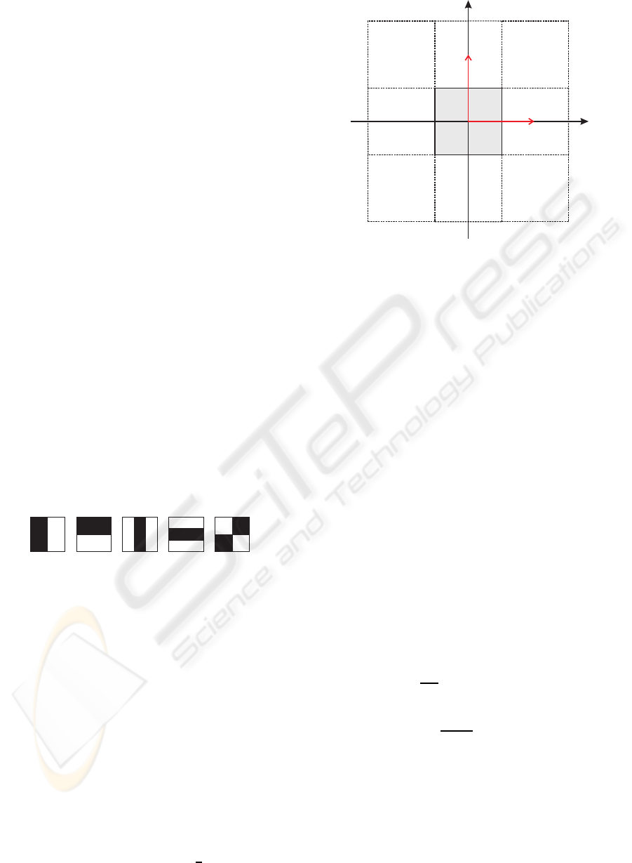
Figure 2: Rectangular sampling in the frequency domain.
Grayish area denotes the rectangular base band and dashed
lines denote the spectral copies. ω
x0
and ω
y0
are the cut-off
frequencies in x- and y- direction respectively. The sam-
pling frequency matrix Ω
Ω
Ω
rect
is constructed using the vec-
tors Ω
Ω
Ω
x
and Ω
Ω
Ω
y
.
where x is the feature vector of an image, h
t
∈ {0,1}
is a weak classifier, α
t
is the weight of the t-th weak
classifier and T is the number of features selected.
The weak classifiers are combined by a weighted ma-
jority vote to a strong classifier H.
After the offline learning process only a few se-
lected features must be calculated for online classifi-
cation.
3 SAMPLING OF 2D SIGNALS
3.1 Naming Conventions and Basics
In the following sections f(x,y) = f (r) denotes a 2D
singal or image with r = (x, y)
T
, where a superscript
T denotes transposition. The same shorthand notation
is used for the Fourier transform.
For a 2D continuous function f(r) the Fourier
transform F( jω
ω
ω)
s c
f(r) with ω
ω
ω = (ω
x
,ω
y
)
T
is de-
fined as
f(r) =
1
(2π)
2
Z
R
2
F( jω
ω
ω)e
jω
ω
ω
T
r
dω
ω
ω (1)
F( jω
ω
ω) =
Z
R
2
f(r)e
− jω
ω
ω
T
r
dr. (2)
3.2 2D Sampling
The transition from 1D to 2D signals, like images,
comes along with new concepts related to sampling.
AN ANALYSIS OF SAMPLING FOR FILTER-BASED FEATURE EXTRACTION AND ADABOOST LEARNING
181
These concepts are caused by the mutual dependen-
cies across different dimensions. In 2D the sampling
period becomes a sampling matrix
T =
T
11
T
12
T
21
T
22
= (T
x
,T
y
).
The sampled signal f
S
(r) and the continuous signal
f (r) are then connected by
f
S
(r) =
∑
n∈Z
2
f (Tn)δ(r− Tn). (3)
In analogy with the 1D case, the relation of the sam-
pling matrix T and the sampling frequency Ω
Ω
Ω is given
by
Ω
Ω
Ω = 2π
T
T
−1
, (4)
where Ω
Ω
Ω is a matrix as well with
Ω
Ω
Ω =
Ω
11
Ω
12
Ω
21
Ω
22
= (Ω
Ω
Ω
x
,Ω
Ω
Ω
y
).
This sampling frequency matrix Ω
Ω
Ω defines where the
spectral copies of the base band are located. Depend-
ing on the spectral properties of the signal at hand an
appropriate sampling scheme can be chosen. In Ohm
(Ohm, 2004) the following sampling schemata are
discussed: rectangular, shear, hexagonal, and quin-
cunx sampling. The simplest option is the rectangu-
lar sampling with a fixed step-width T for both direc-
tions, so that
T = T
1 0
0 1
. (5)
The sampling can be adjusted to the signal properties
for each direction. For example if an image signal has
high frequency components in the x-dimension and a
very fine-grained sampling has to be chosen, this is
not necessarily required for the y-dimension. This is
an important aspect since images are generally resized
preserving the same width to height ratio.
The impact of rectangular sampling with the base
band and its periodic replications are visualized in
figure 2. The width to height ratio is not fixed and
ω
x0
and ω
y0
are the cut-off frequencies in x- and y-
dimension respectively. The resulting sampling fre-
quency is then
Ω
Ω
Ω
rect
=
2ω
x0
0
0 2ω
y0
= (Ω
Ω
Ω
x
,Ω
Ω
Ω
y
).
Using equation 4 the appropriate sampling matrix can
be obtained
T
rect
=
π/ω
x0
0
0 π/ω
y0
.
The difference between 1D and 2D sampling is
that the sampling positions of one dimension can
x
ω
x0
-
x
ω
0
ω
x
ω
y
x
xxx
x
x x x
Ω
y
-
y
ω
0
ω
0y
Ω
x
x x
x
x
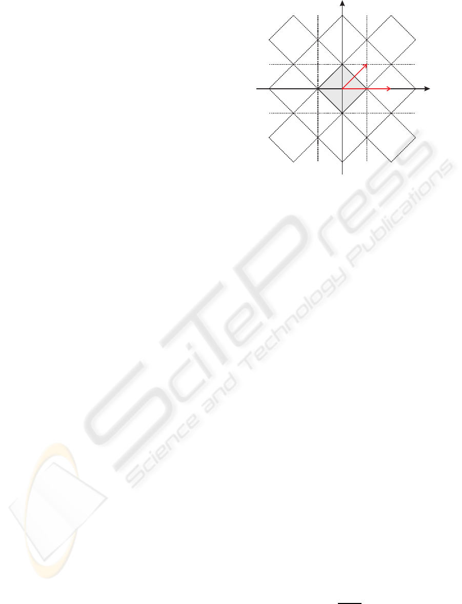
Figure 3: Quincunx sampling in the frequency domain.
Grayish area denotes the rhombus-like base band and
dashed lines denote the spectral copies. ω
x0
and ω
y0
are
the cut-off frequencies in x- and y- direction respectively.
The sampling frequency matrix Ω
Ω
Ω
quin
is constructed using
the vectors Ω
Ω
Ω
x
and Ω
Ω
Ω
y
.
be chosen depending on those of another dimension
(non separable sampling). For example the quincunx
sampling (Ohm, 2004) is a none separable sampling,
where the shape of the base band is rhombus like. Fig-
ure 3 shows a rhombus shaped base band and the ac-
cording periodic replications. It is obvious that one
possible solution to get the sampling frequencymatrix
is to choose Ω
Ω
Ω
x
= (2ω
x0
,0)
T
and Ω
Ω
Ω
y
= (ω
x0
,ω
y0
)
T
.
As a result the sampling frequency is
Ω
Ω
Ω
quin
=
2ω
x0
ω
x0
0 ω
y0
and the corresponding sampling matrix is given by
T
quin
=
π/ω
x0
0
−π/ω
y0
2π/ω
y0
.
3.3 Signal Energy in 2D
Generally, it can be assumed that using sampling
means losing information. To get an idea of how cru-
cial this error is, the energy can be regarded. The en-
ergy of a signal f(r) is defined as
E =
Z
R
2
| f(r)|
2
dr. (6)
Parseval’s theorem (Ohm, 2004) can be used to mea-
sure the energy in the frequency domain
Z
R
2
| f(r)|
2
dr =
1
(2π)
2
Z
R
2
|F( jω
ω
ω)|
2
dω
ω
ω. (7)
With these equations a measure to assess the signal
energy that is preserved in a sampled signal can be
VISAPP 2009 - International Conference on Computer Vision Theory and Applications
182

defined. The energy of the sampled signal can be ap-
proximated by
E
D
=
1
(2π)
2
Z
D
|F( jω
ω
ω)|
2
dω
ω
ω. (8)
D denotes a set which is determined by the cut-off fre-
quencies and the sampling method. For a rectangular
sampling the set can be defined as follows
D
rect
=
ω
x
ω
y
∈ R
2
||ω
x
| ≤ ω
x0
∧ |ω
y
| ≤ ω
y0
.
Analogously a set for the quincunx sampling can be
derived as
D
quin
=
ω
x
ω
y
∈ R
2
|
|ω
x
|
ω
x0
+
|ω
y
|
ω
y0
≤ 1
.
Finally, the energy packing efficiency η
D
of a
sampled signal can be defined as the relative portion
of the energy that is preserved in the sampled signal.
This ratio of energy E
D
and the energy E
ref
of a refer-
ence signal (e.g. the energy E of the continuous sig-
nal) is a measure to compare different sampling rates.
η
D
=
E
D
E
ref
(9)
4 2D SAMPLING FOR IMAGE
FEATURE EXTRACTION
In general, the camera parameters and the distance
in which each training image was collected would be
needed to determine the sampling matrix and thus en-
able the usage of the equations from section 3. For our
experiments it is assumed that this information is not
available. Therefore no information about the sam-
pling period in world coordinates is given and some
assumptions have to be made. It is assumed that the
resolution M × N is the highest possible resolution.
Generally speaking, this is the highest image resolu-
tion that can be found in the trainingset. This image
resolution is used as the reference resolution which is
our optimal case and takes the place of our continuous
signal.
The proposed sampling approach is divided into
two parts. The goal of the first part is to get those pa-
rameters that are necessary to calculate the sampling
matrix in the second part. These are either the number
of sampling points or the energy packing efficiency.
Firstly, a reasonable training resolution M
′
× N
′
has
to be defined. Therefore the approach presented in []
can be used or a fixed resolution can be set in advance
(e.g. 32× 24 for vehicle detection). At this point the
energy packing efficiency for this specific resolution
has to be calculated in reference to M × N using the
equations from section 3. To reach this goal all train-
ing images are resized to the maximal resolution of
M × N and afterwards the mean value of the discrete
Fourier transform (DFT) is calculated. The DFT is
then used in combination with equation 8 and D
rect
to
determine the energy packing efficiency for the reso-
lution M
′
× N
′
. In this context, the cut-off frequencies
are directly connected to the resolution using rectan-
gular sampling. For the maximal resolution the cut-
off frequencies are fixed, so that ω
x0
= π and ω
y0
= π.
The cut-off frequencies ω
′
x0
and ω
′
y0
for a downsam-
pled image are then connected to M
′
× N
′
by
M
′
=
ω
′
x0
M
π
(10)
and
N
′
=
ω
′
y0
N
π
. (11)
Thus, the sampling frequency Ω
Ω
Ω
rect
and the energy
packing efficiency η
D
can be obtained for all resolu-
tions up to M × N.
In the second part an optimized sampling matrix
has to be determined e.g. for quincunx sampling
T
quin
. To find this sampling matrix one of two op-
timization constraints can be chosen. The first one is
to use the energy packing efficiency, so that the new
sampling matrix leads to the same value of η
D
that
was defined in the first part, but using fewer sampling
positions. These positions are distributedaccording to
the signal properties of the images. The second option
is to use the same number of sampling points and find
an arrangement of sampling points that preserve more
energy. In this paper the first option is discussed.
The procedure is almost the same as in part one.
The difference lies in the aspect how the sampling ma-
trix is determined. Now, equation 8 and D
quin
is used
for all different combinations of ω
′
x0
and ω
′
y0
. Thus
for all combinations the energy packing efficiency
can be calculated. Afterwards these values for ω
′
x0
and ω
′
y0
are chosen whoes corresponding energy effi-
ciency value is closest to the predefined value η
D
and
which would result in the lowest number of sampling
points. These sampling periods can then be used to
generate a sampling grid which serves as a rule where
the Haar-like features should be calculated.
5 RESULTS AND CONCLUSIONS
In this section the results provided by the proposed
approach described in the previous sections are dis-
cussed and the performance results of the trained clas-
sifiers are presented. As already mentioned the object
AN ANALYSIS OF SAMPLING FOR FILTER-BASED FEATURE EXTRACTION AND ADABOOST LEARNING
183
detection system developed by Viola & Jones (Viola
and Jones, 2001) is used to verify the approach. The
trainingset consists of 2600 vehicle rear view images
as positive samples and 7007 other images as negative
samples, whereas the independent testset comprises
1114 vehicle rear views and 3003 negative samples.
These manually labeled images are collected from the
Label-Me (Russell et al., 2005) database. To enable
the Haar-like features to capture the edges of the ve-
hicles ten percent of the background is added at the
edges of the images.
For this training- and testset the maximal reso-
lution M × N is 256 × 192, with the same width to
height ratio as presented in (Ponsa et al., 2005). Now
the energy packing efficiency for different resolutions
M
′
× N
′
up to 256 × 192 can be calculated. Fig. 4
shows the energy packing efficiency for progressively
increasing resolution. For a width smaller than 20
pixels the energy is rapidly decreasing, hence choos-
ing a resolution higher than 20× 15 is reasonable. In
this work a training resolution of 32× 24 is chosen,
which is intentionally large compared to other exper-
imental results (e.g. (Ponsa et al., 2005), (Lienhart
et al., 2002)).
0 20 32 100 150 200 250
0.82
0.84
0.86
0.88
0.9
0.92
0.94
0.96
0.98
0.988
1
image width
energy packing efficiency
Figure 4: Energy packing efficiency for progressively in-
creasing resolution.
For this resolution η
D
= 0.988 is obtained, which
means that 98.8% of the energy of the reference im-
age with maximal resolution is preserved. The sam-
pling matrix with reference to 256 × 192 is
T
rect
=
8 0
0 8
.
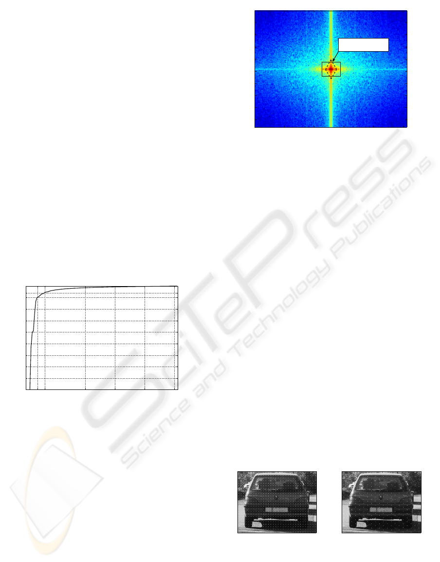
By inspecting the DFT of the training images it be-
comes obvious that the high frequency components
are rather located in the vertical direction (see fig. 5).
This means that our vehicle training images contain
many strong horizontal edges. This fact should be
considered choosing a sampling scheme. It would be
more effective to choose a high resolution in the ver-
tical and a smaller resolution in the horizontal dimen-
sion. This is essentially the outcome of the optimiza-
ω
x
ω
y
50 100 150 200 250
20
40
60
80
100
120
140
160
180
areas containing
98.8% of the energy
Figure 5: Rectangular and Quincunx base band for the train-
ing data preserving 98.8% of the energy. Rectangular and
Quincunx sampling are denoted by the solid and dashed
lines, respectively.
tion procedure from the last section with the quincunx
sampling, where the algorithm is constrained to find a
sampling matrix T which results in preserving 98.8%
of the energy. Regarding the reference resolution, the
optimal sampling scheme is given by
T
quin
=
12.8 0
−6.4 12.8
.
The corresponding base bands for rectangular and
quincunx sampling are shown in figure 5. The quin-
cunx sampling is marked by the dashed line and the
rectangular sampling is marked by the solid line.
Since both methods cover the same energy of the im-
age signals the interesting part is the reduction in sam-
pling points. For the resolution of 32 × 24 the num-
ber of sampling points is 768 and for the quincunx
sampling the number is reduced by more than 50% to
just 300 sampling points. The sampling grids for both
methods are visualized in figure 6. The advantage of
the quincunx sampling is that mutual dependencies
across the x- and y-dimension are considered and that
a higher resolution in vertical than in horizontal di-
mension is achieved.
(a) Rectangular sampling (b) Quincunx sampling
Figure 6: Rectangular (768 sampling points) and Quincunx
(300 sampling points) sampling grid.
For the evaluation, three classifiers are trained us-
ing an AdaBoost algorithm with the same training pa-
VISAPP 2009 - International Conference on Computer Vision Theory and Applications
184
rameters. All classifiers have 100 features and the dif-
ference between these classifiers is the training image
resolution. Two classifiers are trained by resizing the
images to a resolution of 16×12 and 32×24, respec-
tively. For these classifiers the sampling matrix is
T
rect
=
1 0
0 1
.
This sampling matrix is common practice and means
that the five Haar-like features (Fig. 1) are calculated
at all image coordinates.
The third classifier uses the quincunx sampling
method. To perform this sampling, a minimal reso-
lution of 40 × 30 is required. After resizing the im-
age just these positions are used for feature calcula-
tion which are determined by the quincunx sampling
matrix
T
quin
=
2 0
−1 2
.
It is to mention that the minimal size of the Haar-like
features is set to be 2 × 2. Table 1 shows the number
of sampling points and features that are extracted dur-
ing the training process. The performance results of
Table 1: Trained classifiers.
Resolution Sampling Points Features
16× 12, T
rect
192 15· 10
3
32× 24, T
rect
768 260· 10
3
40× 30, T
quin
300 160· 10
3
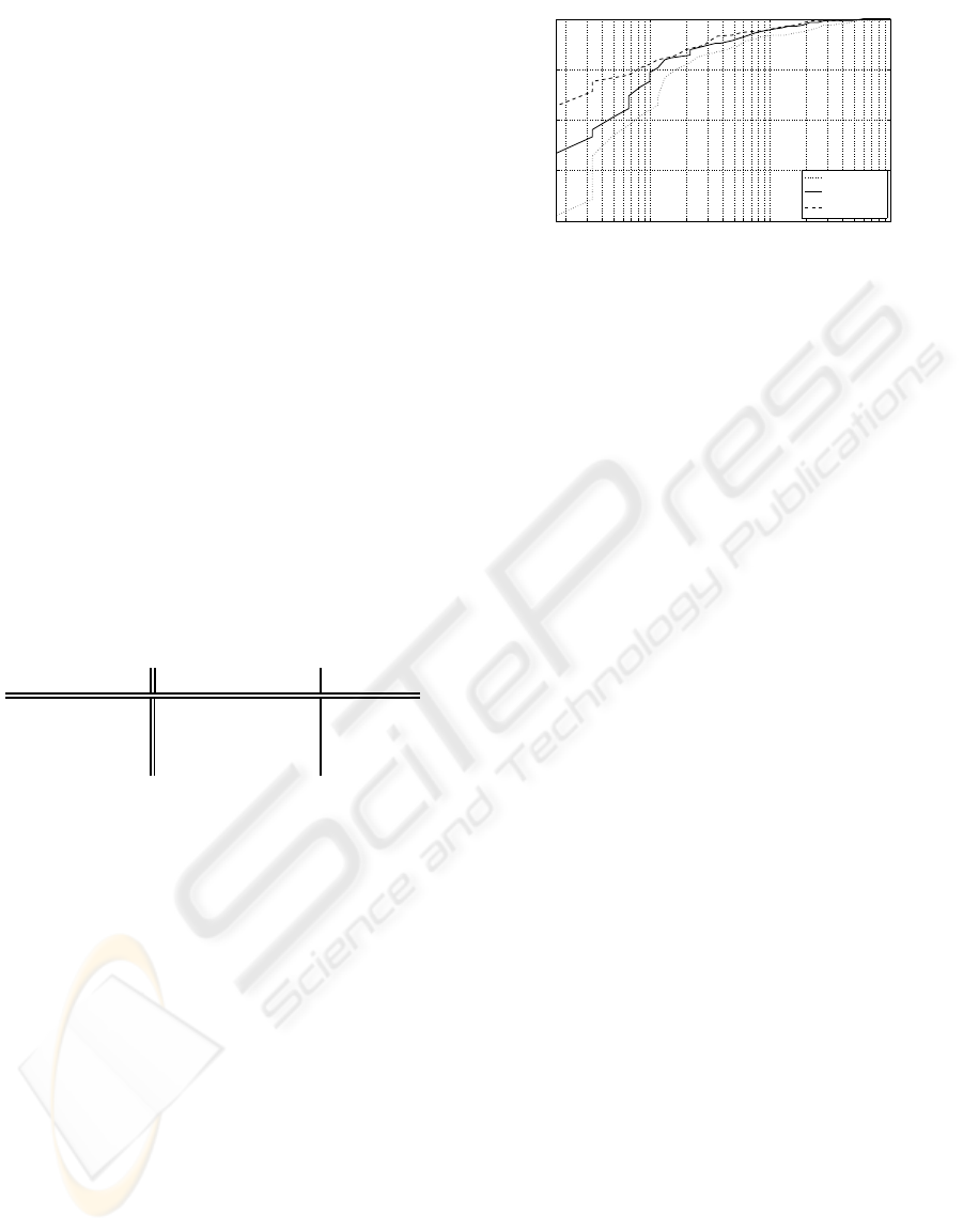
the different classifiers are illustrated by using ROC
curves as shown in Fig. 7. The results reveal that the
best classification performance is obtained by using
the resolution 40 × 30 with the sampling method and
unsatisfying performance by the resolution 16 × 12.
Even though the best classifier’s feature pool is signif-
icantly smaller than the number of features used for
the classifier with resolution 32 × 24 the results are
slightly better. This strengthens the assumption that
the proposed sampling method is valid and moreover
can even improve classification performance without
increasing the computational load during the training
process.
Summing up, an approach has been introduced
to generate a sampling grid to determine reasonable
positions for calculating the Haar-like features. On
the one hand the number of features is reduced by
around 40% and the classification accuracy is in-
creased. These advantages are due to the better uti-
lization of positions for feature calculation which are
adapted to the properties of the training images. One
aspect that should be included in future work is to
transfer this methodology directly to the Haar-like
10
−3
10
−2
10
−1
0.8
0.85
0.9
0.95
1
false positive rate
true positive rate
16x12
32x24
40x30, T
quin
Figure 7: ROC curve of three equally trained classifiers us-
ing two different cartesian and the quincunx sampling.
features to further reduce the computational complex-
ity without losings in accuracy.
REFERENCES
Lienhart, R., Kuranov, A., and Pisarevsky, V. (2002). Em-
pirical analysis of detection cascades of boosted clas-
sifiers for rapid object detection. Technical report,
Mic. Research Lab, Intel Corporation, Santa Clara,
CA 95052, USA.
Ohm, J.-R. (2004). Multimedia Communication Technol-
ogy. Springer, Berlin, Heidelberg, Germany.
Overett, G. and Petersson, L. (2007). Boosting with multi-
ple classifier families. Proc. of IEEE Intelligent Vehi-
cles Symposium, pages 1039–1044.
Ponsa, D., Lopez, A., Lumbreras, F., Serrat, J., and Graf,
T. (2005). 3d vehicle sensor based on monocular vi-
sion. In Proc. of the 8th Int. IEEE Conf. on Intelligent
Transportation Systems, Vienna, Austria.
Russell, B., Torralba, A., and Freeman, W. T. (2005). La-
belme image database. http://labelme.csail.mit.edu.
Sun, Z., Bebis, G., and Miller, R. (2004). On-road vehicle
detection using optical sensors: A review.
Viola, P. and Jones, M. (2001). Rapid object detection us-
ing a boosted cascade of simple features. In Accepted
Conf. on Computer Vision and Pattern Recognition.
AN ANALYSIS OF SAMPLING FOR FILTER-BASED FEATURE EXTRACTION AND ADABOOST LEARNING
185
