AN INVERSE PROBLEM APPROACH TO BRDF MODELING
Kei Iwasaki, Yoshinori Dobashi
Wakayama University, Hokkaido University, Japan
Fujiichi Yoshimoto and Tomoyuki Nishita
Wakayama University, The University of Tokyo, Japan
Keywords:
BRDF(Bidirectional Reflectance Distribution Function), Material Editing, Inverse Problem, Image-based
Lighting.
Abstract:
This paper presents a BRDF modeling method, based on an inverse problem approach. Our method calculates
BRDFs to match the appearance of the object specified by the user. By representing BRDFs by a linear com-
bination of basis functions, outgoing radiances of the object surface can be represented using basis functions.
The calculation of the desired BRDF results from calculating the corresponding coefficients of basis functions
that minimize the sum of differences between the outgoing radiances, represented using basis functions and
user specified radiances. The properties that BRDFs must satisfy are described by linear constraint conditions.
This minimization problem can be solved, interactively, using a linearly constrained least squares approach.
Thus, our method allows the user to design BRDFs directly, under fixed complex lighting and viewpoint, and
to view the rendering results interactively, under dynamic lighting and viewpoint.
1 INTRODUCTION
The research into realistic image synthesis is one of
the most important research topics in computer graph-
ics. The illumination, incident on the objects, and the
reflectance property, described as Bidirectional Re-
flectance Distribution Function (BRDF), are impor-
tant elements in rendering realistic images of objects.
For the applications such as industrial designs, com-
mercial films, movies, and games, designers or direc-
tors often modify the illumination information and/or
the reflectance properties of object surfaces by trial
and error in order to obtain the desired visual effects.
In order to modify the illumination information, sev-
eral methods (Poulin and Fournier, 1992; Schoene-
man et al., 1993; Sloan et al., 2002; Ng et al., 2003;
Hasan et al., 2006; Okabe et al., 2007; Pellacini et al.,
2007) have been proposed.
In recent years, methods of editing BRDFs un-
der fixed illumination have been proposed (Ben-Artzi
et al., 2006; Ben-Artzi et al., 2008). Their methods
decompose the BRDFs into the products of functions
that are represented by 1D parameter. By adjusting
the parameter, interactive editing of BRDFs under en-
vironment illumination can be achieved. Although
these methods can edit BRDFs interactively, trial and
error adjustments of parameters are required to obtain
the images that the user requires.
This paper presents a BRDF modeling method
to permit matching of the desired appearance of ob-
jects under distant lighting represented by an environ-
ment map. Given a fixed illumination condition and
a desired appearance, our method automatically cal-
culates the desired BRDF, based on an inverse prob-
lem approach. This method represents BRDFs by a
linear combination of basis functions. A color of a
pixel, corresponding to a point on the object surface,
can be represented using basis functions and coeffi-
cients corresponding to basis functions. The mod-
eling of BRDFs to match the desired image results
from solving an optimization problem with respect to
coefficients to minimize the difference between the
user specified radiances and the radiances calculated
from the coefficients and the basis functions. In our
method, each object possesses a unique BRDF, but
does not deal with spatially varying BRDFs. The
method deals with all-frequency lighting, represented
by an environment map. The method does not mod-
ify the illumination conditions, (for example, adding
local point light sources to add highlights), since the
modification of the illumination conditions can affect
129
Iwasaki K., Dobashi Y., Yoshimoto F. and Nishita T. (2009).
AN INVERSE PROBLEM APPROACH TO BRDF MODELING.
In Proceedings of the Fourth International Conference on Computer Graphics Theory and Applications, pages 129-136
DOI: 10.5220/0001784601290136
Copyright
c
 SciTePress

all the synthesized objects, and therefore, it is difficult
to modify the appearance of a particular object.
This paper is organized as follows. Section 2 re-
views previous work. Section 3 describes our inverse
BRDF modeling method. Section 4 explains the im-
plementation details. Section 5 shows some results
of the rendering process, and the conclusions to this
work are brought together in Section 6.
2 PREVIOUS WORK
We first review previous methods for pre-computed
radiance transfer (PRT), since our method is related
to PRT methods. Then previous methods of BRDF
editing are discussed.
2.1 Pre-computed Radiance Transfer
(PRT)
Pre-computation-based techniques have been devel-
oped for fast re-lighting. Dobashi et al. (Dobashi
et al., 1995) proposed a method that used spherical
harmonics to achieve fast re-lighting for interactive
lighting design. Moreover, Dobashi et al. (Dobashi
et al., 1996) used Fourier series to represent the in-
tensity distributions at the surfaces of objects, illumi-
nated by the sky. Ramamoorthi and Hanrahan (Ra-
mamoorthi and Hanrahan, 2002) proposed a real-time
rendering method for environment illumination, us-
ing spherical harmonics. Sloan et al. (Sloan et al.,
2002) proposed a PRT technique for real-time render-
ing under environment illumination using the spher-
ical harmonics as the basis functions. Several meth-
ods (Kautz et al., 2002; Lehtinen and Kautz, 2003;
Sloan et al., 2003a; Sloan et al., 2003b; Sloan et al.,
2005) have been proposed to extend the PRT method.
These PRT methods basically focus on the changes
in the viewpoint and the illumination at run-time. A
change in the BRDF at run-time is possible, but a
large volume of pre-computed BRDF data is required.
Ng et al. (Ng et al., 2003) used wavelet basis
functions for a non-linear lighting approximation and
achieved interactive rendering for diffuse surfaces.
Several methods (Wang et al., 2004; Liu et al., 2004;
Tsai and Shih, 2006) have been proposed to render
glossy surfaces. Although these methods can create
realistic images in an all-frequency lighting environ-
ment, they require pre-computed BRDF data and ren-
dering it is quite difficult to arbitrarily change BRDFs
at run-time. Okabe et al. (Okabe et al., 2007) pro-
posed an appearance-based illumination design sys-
tem based on PRT techniques. This method, however,
focuses on the design of illumination, not BRDFs.
In recent years, PRT methods for calculating dy-
namic BRDFs have been proposed. Sun et al. (Sun
et al., 2007) proposed a PRT method for dynamic
BRDFs. This method compresses the pre-computed
BRDF data by using tensor decompositions, and cal-
culates the pre-computedtransfer tensors (PTT). Then
interactive rendering with dynamic viewpoint, light-
ing and BRDFs can be achieved by using the PTTs.
This method, however, requires the pre-computed
BRDF data and it is difficult to change the BRDF that
is not included in the pre-computed BRDF data.
2.2 BRDF Editing
Ben-Artzi et al. (Ben-Artzi et al., 2006) proposed
a real-time BRDF editing method under an all-
frequency illumination environment. This method
can edit the BRDFs by changing the parameters, such
as the glossiness of the Phong BRDF. Akerlund et
al. (Akerlund et al., 2007) proposed a precomputed
visibility cuts for relighting static scenes with dy-
namic BRDFs. These methods, however, require trial
and error adjustments of the parameters, to obtain the
desired images.
Colbert et al. (Colbert et al., 2006) proposed a
method that models the BRDFs by drawing the high-
lights on a spherical canvas. This method approxi-
mates the highlights by using Ward BRDFs (Ward,
1992). This method, however, cannot create high-
lights, directly, on a user-specified region of the object
surface.
Ashikhmin et al. (Ashikhmin et al., 2000) pro-
posed a method to generate BRDFs by inputting a 2D
micro-facet orientation distribution. Jaroszkiewicz
and McCool (Jaroskiewicz and McCool, 2003) pro-
posed a method to extract BRDFs and material
maps from images using homomorphic factorization.
Lawrence et al. (Lawrence et al., 2006) proposed an
inverse shade tree framework that decomposes spa-
tially varying BRDFs (SVBRDFs) into 1D editable
functions. These methods, however, are limited to
a point light source. Pellacini et al. (Pellacini and
Lawrence, 2007) proposed an editing method for spa-
tially and temporally varying BRDFs. This method,
however, does not consider the complex illumination.
Khan et al. (Khan et al., 2006) proposed an image-
based material editing method that transforms a pho-
tograph of an object into a photograph of the object
whose material is changed. Although this method
can change the appearance of the object surface, this
method cannot calculate the optimal BRDF to mach
the images that the user requires. Ngan et al. (Ngan
et al., 2006) proposed a visual navigation system
of analytical BRDF models under complex lighting.
GRAPP 2009 - International Conference on Computer Graphics Theory and Applications
130

(a) initial state (b) user specifies regions (c) rendering result
(car body is diffuse BRDF) (white strokes) to add highlights using modeled BRDF
Figure 1: These figures show the overview of our method. The left image (a) shows the car body with diffuse BRDF as the
initial state. As shown in the center image (b), the user paints strokes where the user wants to add highlights or change colors.
Our method models the BRDF so as to create highlights in the regions specified by the user. The right image (c) shows the
result that is rendered by using the calculated BRDF. The computational time of the BRDF in (c) is 0.26 sec. As shown in (c),
our method can obtain the BRDF to match the appearance the user requested interactively.
This method, however, does not model the desired
BRDF. Recently, Pacanowskiet al. (Pacanowski et al.,
2008) proposed a sketch-based interface for highlight
modeling. This method, however, is not applied to
complex lighting. To address these problems, we pro-
pose a calculation method for BRDFs that fit the user-
specified radiances by using an inverse problem ap-
proach.
3 PROPOSED INVERSE BRDF
MODELING
3.1 Overview
Outgoing radiance, B(x,ω
o
), at point, x, in direc-
tion, ω
o
, under environment illumination is calculated
from the following equation:
B(x,ω
o
) =
Z
Ω
L(ω
i
)V(x,ω
i
) f
r
(ω
i
,ω
o
)(ω
i
· n(x))dω
i
, (1)
where Ω is the direction on the hemisphere, ω
i
is
the incident direction, L(ω
i
) is the source radiance,
V(x,ω
i
) is the visibility function, f
r
(ω
i
,ω
o
) is the
BRDF, and n(x) is the normal vector at x (see Fig. 2).
To simplify the notation, the dot product (ω
i
· n(x))
is included in the visibility function V(x,ω
i
), and
˜
V(x,ω
i
) is defined as
˜
V(x,ω
i
) = V(x,ω
i
)(ω
i
· n(x)).
In our method, BRDF f
r
is represented with a sum
of diffuse term f
d
and specular term f
s
as follows:
f
r
(ω
i
,ω
o
) = f
d
+ f
s
(ω
i
,ω
o
). (2)
The diffuse term f
d
is represented with f
d
= ρ
d
/π,
where ρ
d
is the diffuse albedo. The component B
d
(x)
of the outgoing radiance corresponding to the diffuse
term f
d
is calculated from:
B
d
(x) =
Z
Ω
L(ω
i
)
˜
V(x,ω
i
)
ρ
d
π
dω
i
= ρ
d
E(x), (3)
where E(x) is the irradiance at x. To model the dif-
fuse term f
d
simply and efficiently, the diffuse albedo
ρ
d
is directly specified by the user.
Our method represents the specular term
f
s
(ω
i
,ω
o
) by a product of a linear combination
of basis functions and the static function s of the
incident and outgoing directions (the static function s
is described in Section 3.2):
f
s
(ω
i
,ω
o
) = s(ω
i
,ω
o
)
J−1
∑
j=0
c
j
φ
j
(ω
i
,ω
o
), (4)
where c
j
is j-th coefficient, corresponding to j-th ba-
sis function, φ
j
, and J is the number of basis func-
tions. By substituting Eq. (4) into Eq. (1), the compo-
nent B
s
(x,ω
o
) of the outgoing radiance corresponding
to the specular term f
s
is rewritten as:
B
s
(x,ω
o
(x))
=
Z
Ω
L(ω
i
)
˜
V(x,ω
i
)
J−1
∑
j=0
c
j
φ
j
(ω
i
,ω
o
)s(ω
i
,ω
o
)
!
dω
i
=
J−1
∑
j=0
c
j
Z
Ω
L(ω
i
)
˜
V(x,ω
i
)φ
j
(ω
i
,ω
o
)s(ω
i
,ω
o
)dω
i
.
(5)
When modeling BRDFs, we assume that the view-
point and the object surfaces are fixed
1
. Under this
assumption, the viewing direction, ω
o
, depends on the
position, x, and is represented by ω
o
(x).
In this equation, we define the transfer function
T
j
(x) as:
T
j
(x)=
Z
Ω
L(ω
i
)
˜
V(x, ω
i
)φ
j
(ω
i
,ω
o
(x))s(ω
i
,ω
o
(x))dω
i
. (6)
Using T
j
(x), the component B
s
(x), is calculated from:
B
s
(x) =
J−1
∑
j=0
c
j
T
j
(x). (7)
1
Our method can deal with modeling the BRDFs with
multiple viewpoints, by solving Eq. (7) using transfer func-
tions of multiple viewpoints.
AN INVERSE PROBLEM APPROACH TO BRDF MODELING
131

x
n(x)
ω
o
(x)
ω
i
screen
viewpoint
L(
ω
i
)
source radiance
object surface
Figure 2: Outgoing radiance calculation.
Let the pixels corresponding to the object surface
be X = {x
0
,x
1
,· ·· ,x
N−1
} (N is the number of pixels
corresponding to the object surface), with the colors
B = {B
0
,B
1
,· ·· ,B
N−1
} at these pixels. The colors are
specified by the users by painting strokes, and the de-
tails are described in Section 4.3. A desired BRDF of
the specular term is obtained by calculating the coef-
ficients, c
j
, for each object to minimize the following
equation:
argmin
c
j
N−1
∑
i=0
(B
i
−
J−1
∑
j=0
c
j
T
j
(x
i
))
2
. (8)
In solving the optimization problem expressed by
Eq. (8), we have to take into account the following
BRDF properties.
• Helmholtz reciprocity
• energy conservation
• non-negativity
The Helmholtz reciprocity is represented by the fol-
lowing equation:
f
r
(ω
i
,ω
o
) = f
r
(ω
o
,ω
i
). (9)
The energy conservationis represented by the follow-
ing equation:
Z
Ω
f
r
(ω
i
,ω
o
)(ω
i
· n)dω
i
≤ 1 ∀ω
o
. (10)
Non-negativity states that f
r
(ω
i
,ω
o
) ≥ 0 for any ω
i
and ω
o
.
In the next section, basis functions that are suited
to represent specular term and to satisfy the BRDF
properties are described.
3.2 Basis Functions to Represent
BRDFS
BRDFs are, in general, four dimensional functions
(two dimensions for the incident direction and two
dimensions for the outgoing direction), and require
a large number of basis functions to be repre-
sented. This results in increasing the pre-computation
data, thus decreasing the rendering frame rates. To
represent BRDFs with a small number of basis
n
ω
i
ω
o
h
θ
h
normal vector
tangent vector
binormal vector
Figure 3: Half vector.
functions, our method employs Distribution-based
BRDFs (Ashikhmin, 2006). The distribution-based
BRDF model is calculated from the following equa-
tion:
f
s
(ω
i
,ω
o
) =
p(h)F(ω
i
· h)
(ω
i
· n) + (ω
o
· n) − (ω
i
· n)(ω
o
· n)
, (11)
where h is the half vector of ω
i
and ω
o
, calcu-
lated from h = (ω
i
+ ω
o
)/||(ω
i
+ ω
o
)|| (see Fig. 3).
p(h) is the distribution function of the half vector,
F(ω
i
· h) is the Fresnel term, and n is the normal vec-
tor. Since h is reciprocal for any ω
i
and ω
o
, f
r
sat-
isfies Helmholtz reciprocity for any function p. In
the distribution-based BRDF model, the reflectance
property is mainly affected by the distribution func-
tion p(h). Therefore, our method represents the dis-
tribution function, p(h), by a linear combination of
basis functions, φ
j
(h), as p(h) =
∑
j=0
c
j
φ
j
(h), and
the other factor, F(ω
i
· h)/((ω
i
· n) + (ω
o
· n) − (ω
i
·
n)(ω
o
· n)), is the static function s in Eq. (4).
Our method represents the distribution function,
p(h), by basis functions, φ
j
(h). In the previous
PRT methods (Sloan et al., 2002; Ng et al., 2003),
orthogonal basis functions, such as spherical har-
monics and Haar wavelets, are used to approximate
functions. In our method, orthogonality is not nec-
essary and the method only needs a small num-
ber of basis functions to approximate the distribu-
tion function efficiently. The distribution functions
for analytic BRDF models tend to have sharp peaks
to represent highlights. Therefore, our method re-
quires basis functions, φ
j
(h), that can represent high-
frequency functions with sharp peaks. Spherical har-
monics are suited to represent low-frequency func-
tions, but a large number of functions is required to
represent high-frequency functions. We also consid-
ered Haar wavelets (Ng et al., 2003) and Daubechies
wavelets (Ben-Artzi et al., 2006) that are often used
to represent high-frequency functions, but Haar and
Daubechies wavelets can take negative values. To sat-
isfy the non-negativity of the BRDF, it is sufficient
to satisfy condition p(h) > 0 for all h, since the de-
nominator of the distribution BRDF and the Fresnel
term are non-negative for any ω
i
and ω
o
. However,
GRAPP 2009 - International Conference on Computer Graphics Theory and Applications
132

if wavelets are used to represent the distribution func-
tion, many constraint conditions for coefficients, c
j
,
are required to satisfy the non-negativity for any ω
i
and ω
o
. This results in increased calculation time of
coefficients, c
j
.
To represent the distribution function, p(h),
our method uses spherical radial basis functions
(SRBF) (Tsai and Shih, 2006) as
p(h) ≈
J−1
∑
j=1
c
j
G(h· ξ
j
,λ), (12)
where G is the Gaussian SRBF, ξ
j
is the center of j-th
SRBF and λ is the bandwidth parameter of SRBF.
The reasons for using SRBFs are as follows.
Firstly, high-frequency functions can be represented
by using a small number of SRBFs, as described in
(Tsai and Shih, 2006). Secondly, the constraint con-
ditions for the non-negativity of the distribution func-
tion can be described easily by the SRBFs. Since
SRBFs are non-negative function for any half vector
h, (that is for any ω
i
and ω
o
), the constraint condition
for the non-negativity is simply described as c
j
≥ 0.
The energy conservation condition of the sum of
diffuse term f
d
and specular term f
s
is represented as:
Z
Ω
( f
d
+ f
s
(ω
i
,ω
o
))(ω
i
· n)dω
i
≤ 1. (13)
In Eq. (13), the integration of the diffuse term f
d
=
ρ
d
π
is computed as
R
Ω
ρ
d
π
(ω
i
· n)dω
i
= ρ
d
.
To satisfy the energy conservationcondition of the
specular term for any ω
o
, we discretize N
l
directions
on the hemisphere. Then our method calculates the
integration in Eq. (10) for each discretized outgoing
directions, ω
l
o
(0 ≤ l ≤ N
l
− 1):
ρ
d
+
Z
Ω
J−1
∑
j=0
c
j
G(h· ξ
j
,λ)s(ω
i
,ω
l
o
)dω
i
≤ 1. (14)
In Eq. (14), we define the integrated values for each
discretized outgoing direction, ω
l
o
as g
l
j
:
g
l
j
=
Z
Ω
G(h· ξ
j
,λ)s(ω
i
,ω
l
o
)dω
i
. (15)
Then the energy conservation conditions for N
l
dis-
cretized directions are described as:
J−1
∑
j=0
g
l
j
c
j
≤ 1− ρ
d
(0 ≤ l ≤ N
l
− 1). (16)
Consequently, our method calculates the coeffi-
cient vector, c = (c
0
,c
1
,· ·· ,c
J−1
), that minimizes:
N−1
∑
i=0
(B
i
−
J−1
∑
j=0
c
j
T
j
(x
i
))
2
, (17)
while satisfying the following linear constraint con-
ditions:
c
j
≥ 0 (0 ≤ j ≤ J − 1), (18)
J−1
∑
j=0
g
l
j
c
j
≤ 1− ρ
d
(0 ≤ l ≤ N
l
− 1). (19)
4 IMPLEMENTATION DETAILS
4.1 Precomputation
Our method pre-computes the transfer function,
T
j
(x), at each point, x, corresponding to each pixel of
the screen. The computational time for the coefficient
vector, c, depends on the number of corresponding
pixels, N (see Eq. (8)). If the screen size is 640× 480,
N is about 300,000 and the computational time of c
becomes enormous. To calculate c interactively, our
method prepares a low-resolution screen of the frame
buffer. Then the least squares problem with linear
constraint conditions is solved using down-sampled
images. In our experiments, the size of down-sampled
images is set to 160 × 120 for the 640 × 480 screen,
and this works well for all our examples.
The transfer function at each pixel is then com-
puted. To compute the transfer function described in
Eq. (6), a large number of uniformly distributed di-
rections on the sphere are prepared. Then the integra-
tion in Eq. (6) is calculated by summing the product
of functions L,
˜
V, φ
j
and s evaluated at each direc-
tion. This calculation, however, is time-consuming
since the number of directions is quite large.
To compute the transfer function efficiently, our
method employs the precomputed visibility cuts
method proposed by (Akerlund et al., 2007). In gen-
eral, the cosine-weighted visibility function
˜
V has
large coherent regions. Therefore, the directions on
the sphere can be partitioned into a small number of
clusters, where
˜
V can be approximated by a piece-
wise constant function. The cosine-weighted visibil-
ity function in the k-th cluster C
k
is approximated by
the mean cluster value hv
k
i:
hv
k
(x)i =
1
|C
k
|
∑
˜
V(x, ω
i
),ω
i
∈ C
k
. (20)
The transfer function T
j
(x) can be computed effi-
ciently as:
T
j
(x) =
∑
k
|C
k
|L(ω
k
)hv
k
(x)i
˜
φ
j
(h
k
), (21)
where ω
k
is the representative direction of cluster C
k
,
˜
φ
j
is the j-th basis function multiplied with the static
function, and h
k
is the half vector of ω
k
and viewing
direction ω
o
(x).
To compute the mean cluster value hv
k
(x)i at sur-
face point x corresponding to each pixel, our method
precomputes each cluster value at each vertex x
v
of
the triangles of the object surface. Then the mean
cluster value hv
k
(x)i at x is computed by interpolat-
ing the precomputed cluster values at three vertices of
the triangle that contains surface point x.
AN INVERSE PROBLEM APPROACH TO BRDF MODELING
133

4.2 BRDF Modeling and Rendering
Our method calculates the coefficient vector, c, that
minimizes Eq. (17). This coefficient vector can be
obtained by solving the least squares problem with
linearly constrained conditions, using Numerical Al-
gorithm Group library (NAG, 2007). Our method also
allows the users to create a BRDF that is physically
impossible by ignoring the linearly constrained con-
ditions, if the users want.
After the coefficient vector c is obtained, our
method calculates the outgoing radiance at each ver-
tex by using Eq. (5). To allow the users to change
the viewpoint and the illumination, our method calcu-
lates Eq. (5) on the fly. To compute Eq. (5) efficiently,
our method uses the precomputed visibility cuts. The
outgoing radiance B(x
v
,ω
o
) at vertex x
v
is calculated
from:
B(x
v
,ω
o
) =
∑
k
L(ω
k
)hv
k
(x
v
)i(
ρ
d
π
+
∑
j
c
j
˜
φ
j
(h
k
)). (22)
The calculation of the radiance at each vertex ex-
pressed in Eq. (22) is performed on the GPU as de-
scribed in (Akerlund et al., 2007).
4.3 Interface
Our method specifies the colors by painting strokes
on the image directly. The strokes are represented as
point sequences. The brush to paint strokes has four
parameters: color C, diameter D, gaussian parame-
ter κ and scaling factor S. The specified color B
i
of
pixel x
i
using colorC is calculated from the following
equation:
B
i
= w
i
C+(1− w
i
)B
′
i
,
w
i
=

exp(−κd
i
) d
i
≤ D
0 d
i
> D
, (23)
where d
i
is the distance between x
i
and the stroke, B
′
i
is the color of pixel x
i
before painting. The users can
also specify the color B
i
by using the scaling factor S
(S ≥ 0) and the color B
′
i
as B
i
= w
i
SB
′
i
+ (1− w
i
)B
′
.
Not only creating highlights, our method also can
delete highlights by assigning negative values to C.
5 RESULTS
We have tested our algorithm on a standard PC
equipped with Core2Quad 2.66GHz CPU with 3GB
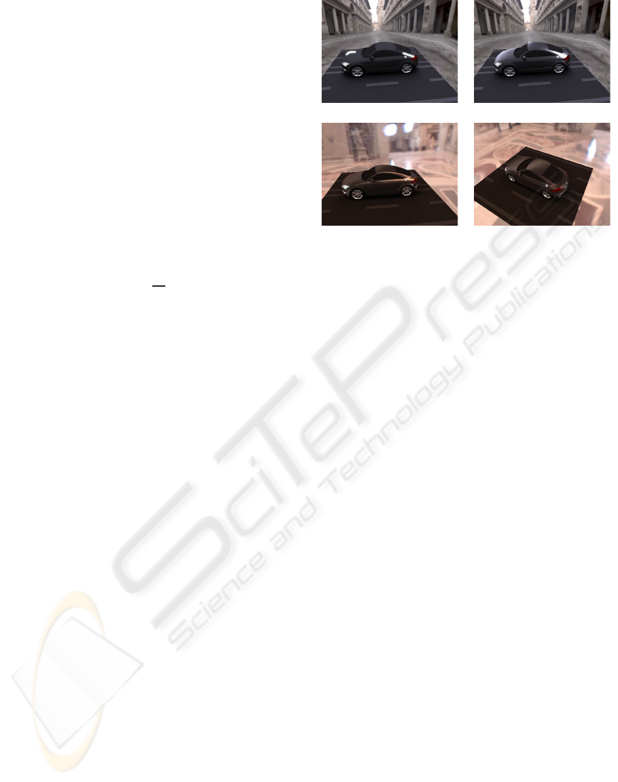
memory and a GeForce 8800 GTX. Fig. 4 shows im-
ages of a car model with BRDFs modeled by using
our method. Fig. 4(a) shows the user specified white
strokes and Fig. 4(b) shows the rendering result us-
ing the modeled BRDF that brightens the specified
regions. Figs. 4(c) and (d) show the rendering results
(a) initial state and strokes (b) rendering result
(c) relighting (d) changing viewpoint
Figure 4: A car model with BRDFs modeled by using our
method. The precomputation time of visibility cuts is 70
minutes. The data size of precomputed visibility cuts is 123
MB. The average number of clusters is about 200..
using the BRDF in (b) under different lighting and
viewpoint. Fig. 5 shows images of a bunny model.
Figs. 5(a) and (c) show the initial states and strokes
and Figs. 5(b) and (d) show the rendering results, re-
spectively. The calculated BRDFs are visualized in
lower left of Figs. 5(b) and (d). The yellow arrow
shows the incident direction.
Fig. 6 shows images of a room scene. Highly
specular BRDF is modeled in the left modern chair,
and dim highlight is created in the right antique chair.
Our method sets each center of SRBF, ξ
j
, to
each direction corresponding to each pixel of the
hemicube. That is, the number (J) of basis functions
to represent the specular term is 147(3 × 7 × 7) in
our examples. The bandwidth parameter λ is calcu-
lating the relationship between the variance σ and λ
:σ
2
= 1− (cosh(2λ)−(2λ)
−1
) (Narcowich and Ward,
1996). We set σ to π/40 and this works well in our
examples. The number of the discretized direction (N
l
in Eq. (16)), is set to 192.
Table 1 shows the statistics of our method. As
shown in Table 1, our method can show the calculated
BRDF immediately. Moreover,our method allows the
users to relight the scene and change the viewpoint
interactively. These interactive feedbacks are helpful
for the users to model BRDFs intuitively.
The limitation of our method is as follows. Al-
though our method calculates the BRDFs as much
as possible to match the appearance specified by the
user, the radiances of regions where the user does not
specify may also change. The regions whose transfer
functions are similar to those at specified regions tend
to be affected. This can be relaxed by weighting the
GRAPP 2009 - International Conference on Computer Graphics Theory and Applications
134

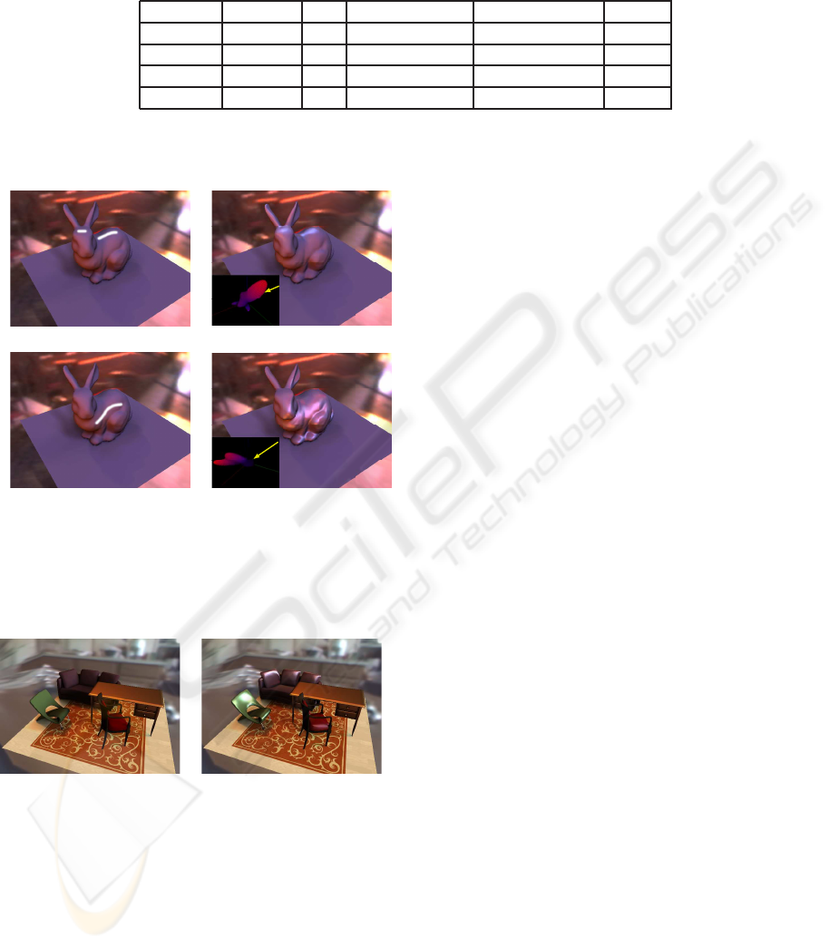
Table 1: Statistics of our method. T
s
represents the computational time to solve a least squares problem. N is the number of
pixels corresponding to the object surface in the 160× 120 image. T
trans
indicates the computational time of transfer functions
at N pixels. In Fig. 6, T
s
and N for sofa/left chair/cushion of the right chair are listed. T
trans
in Fig. 6 shows the total time to
compute transfer functions of three objects.
Fig. No. Vertices fps T
s
N T
trans
Fig. 1 77K 2.2 0.26 sec 2656 28 sec
Fig. 4 77K 2.2 0.17 sec 1797 24 sec
Fig. 5 22K 2.3 0.14 sec 1299 22 sec
Fig. 6 117K 0.7 0.22/0.11/0.04 2066/1092/460 55 sec
values of transfer functions in Eq. (17).
(a) initial state and strokes (b) result
(c) initial state and strokes (d) result
Figure 5: The bunny model with BRDFs modeled by using
our method. The precomputation time of visibility cuts is 4
minutes. The data size of precomputed visibility cuts is 53
MB. The average number of clusters is about 300..
(a) initial state (b) result
Figure 6: The room scene with BRDFs modeled by using
our method. The precomputation time of visibility cuts is
54 minutes. The data size of precomputed visibility cuts is
279 MB. The average number of clusters is about 332.
6 CONCLUSIONS
We have proposed an appearance-based BRDF mod-
eling method, using an inverse problem approach. By
representing BRDFs by a linear combination of basis
functions, the outgoing radiances can be represented
with a linear combination of transfer functions, cal-
culated using basis functions. The method solves the
optimization problem to minimize the sum of the dif-
ferences between the outgoing radiances calculated
from the transfer functions and the radiances speci-
fied by the user. Our method solves this problem by
satisfying the BRDF properties: reciprocity, energy
conservation, and non-negativity. The method allows
the user to model the desired BRDF interactively and
intuitively.
In future, we intend to calculate, not only the de-
sired BRDFs, but also the optimal illumination infor-
mation, to obtain desired images.
REFERENCES
Akerlund, O., Unger, M., and Wang, R. (2007). Precom-
puted visibility cuts for interactive relighting with dy-
namic BRDFs. In Proceedings of Pacific Graphics
2007, pages 161–170.
Ashikhmin, M. (2006). Distribution-based BRDFs. In
http://jesper.kalliope.org/blog/library/dbrdfs.pdf.
Ashikhmin, M., Premoze, S., and Shirley, P. (2000). A
microfacet-based BRDF generator. In Proceedings of
SIGGRAPH 2000, pages 65–74.
Ben-Artzi, A., Egan, K., Ramamoorthi, R., and Durand,
F. (2008). A precomputed polynomial representation
for interactive BRDF editing with global illumination.
ACM Transactions on Graphics, 27(2):13.
Ben-Artzi, A., Overbeck, R., and Ramamoorthi, R. (2006).
Real-time BRDF editing in complex lighting. ACM
Transaction on Graphics, 25(3):945–954.
Colbert, M., Pattanaik, S., and Krivanek, J. (2006). BRDF-
shop: Creating physically correct bidirectional re-
flectance distribution functions. IEEE Computer
Graphics and Applications, 26(1):30–36.
Dobashi, Y., Kaneda, K., Yamashita, H., and Nishita, T.
(1995). A quick rendering method using basis func-
tions for interactive lighting design. Computer Graph-
ics Forum, 14(3):229–240.
Dobashi, Y., Kaneda, K., Yamashita, H., and Nishita, T.
(1996). Method for calculation of sky light luminance
AN INVERSE PROBLEM APPROACH TO BRDF MODELING
135

aiming at an interactive architectural design. Com-
puter Graphics Forum, 15(3):112–118.
Hasan, M., Pellacini, F., and Bala, K. (2006). Direct-to-
indirect transfer for cinematic relighting. ACM Trans-
action on Graphics, 25(3):1089–1097.
Jaroskiewicz, R. and McCool, M. D. (2003). Fast extrac-
tion of BRDFs and material maps from images. In
Proceedings of Graphics Interface 2003, pages 1–10.
Kautz, J., Sloan, P., and Snyder, J. (2002). Fast, arbi-
trary BRDF shading for low-frequency lighting using
spherical harmonics. In Proc. Eurographics Workshop
on Rendering 2002, pages 301–308.
Khan, E. A., Reinhard, E., Fleming, R. W., and Bulthoff,
H. H. (2006). Image-based material editing. ACM
Transactions on Graphics, 25(3):654–663.
Lawrence, J., Ben-Artzi, A., DeCoro, C., Matusik, W.,
Pfister, H., Ramamoorthi, R., and Rusinkiewicz, S.
(2006). Inverse shade trees for non-parametric ma-
terial representation and editing. ACM Transactions
on Graphics, 25(3):735–745.
Lehtinen, J. and Kautz, J. (2003). Matrix radiance transfer.
In Proc. Symposium on Interactive 3D Graphics 2003,
pages 59–64.
Liu, X., Sloan, P., Shum, H., and Snyder, J. (2004). All-
frequency precomputed radiance transfer for glossy
objects. In Proc. Eurographics Symposium on Ren-
dering 2004, pages 337–344.
NAG (2007). Numerical algorithm group c library.
Narcowich, F. J. and Ward, J. D. (1996). Nonstationary
wavelets on them-sphere for scattered data. Applied
and Computational Harmonic Analysis, 3(4):324–
336.
Ng, R., Ramamoorthi, R., and Hanrahan, P. (2003). All-
frequency shadows using non-linear wavelet light-
ing approximation. ACM Transactions on Graphics,
22(3):376–381.
Ngan, A., Durand, F., and Matusik, W. (2006). Image-
driven navigation of analytical BRDF models. In Pro-
ceedings of Eurographics Symposium on Rendering
2006, pages 399–408.
Okabe, M., Matsushita, Y., Shen, L., and Igarashi, T.
(2007). Illumination brush: Interactive design of all-
frequency lighting. In Proceedings of Pacific Graph-
ics 2007, pages 171–180.
Pacanowski, R., Grainer, X., Schick, C., and Poulin, P.
(2008). Sketch and paint-based interface for high-
light modeling. In Eurographics Workshop on Sketch-
Based Interfaces and Modeling.
Pellacini, F., Battaglia, F., Morley, R., and Finkelstein, A.
(2007). Lighting with paint. ACM Transactions on
Graphics, 26(2):9.
Pellacini, F. and Lawrence, J. (2007). Appwand: Edit-
ing measured materials using appearance-driven op-
timization. ACM Transactions on Graphics, 26(3):54.
Poulin, P. and Fournier, A. (1992). Lights from highlights
and shadows. In Proceedings of Symposium on Inter-
active 3D Graphics 1992, pages 31–38.
Ramamoorthi, R. and Hanrahan, P. (2002). Frequency space
environment map rendering. ACM Transactions on
Graphics, 21(3):517–526.
Schoeneman, C., Dorsey, J., Smits, B., Arvo, J., and Green-
berg, D. (1993). Painting with light. In Proceedings
of SIGGRAPH’93, pages 143–146.
Sloan, P., Hall, J., Hart, J., and Snyder, J. (2003a). Clus-
tered principal components for precomputed radiance
transfer. ACM Transactions on Graphics, 22(3):382–
391.
Sloan, P., Kautz, J., and Snyder, J. (2002). Precomputed
radiance transfer for real-time rendering in dynamic
scenes. ACM Transactions on Graphics, 21(3):527–
536.
Sloan, P., Liu, X., Shum, H., and Snyder, J. (2003b). Bi-
scale radiance transfer. ACM Transactions on Graph-
ics, 22(3):370–375.
Sloan, P., Luna, B., and Snyder, J. (2005). Local, de-
formable precomputed radiance transfer. ACM Trans-
actions on Graphics, 24(3):1216–1224.
Sun, X., Zhou, K., Chen, Y., Lin, S., Shi, J., and Guo, B.
(2007). Interactive relighting with dynamic BRDFs.
ACM Transaction on Graphics, 26(3):27.
Tsai, Y.-T. and Shih, Z.-C. (2006). All-frequency precom-
puted radiance transfer using spherical radial basis
functions and clustered tensor approximation. ACM
Transaction on Graphics, 25(3):967–976.
Wang, R., Tran, J., and Luebke, D. (2004). All-
frequency relighting of non-diffuse objects using sep-
arable BRDF approximation. In Proc. Eurographics
Symposium on Rendering 2004, pages 345–354.
Ward, G. J. (1992). Measuring and modeling anisotropic
reflection. ACM SIGGRAPH Compute Graphics,
26(2):265–272.
GRAPP 2009 - International Conference on Computer Graphics Theory and Applications
136