SEMI-AUTOMATIC PARTITIONING BY VISUAL SNAPSHOPTS

Rosa Matias

, João-Paulo Moura

2, 4

, Paulo Martins

2, 4

and Fátima Rodrigues

3, 4

Polytechnic Institute of Leiria, Morro do Lena - Alto Vieiro, Leiria, Portugal

Department of Engineer, University Of Trás-os-Montes e Alto Douro, Vila Real, Portugal

Department of Informatics, Porto Institute of Engineering, Porto, Portugal

Knowledge Engineering and Decision Support Research Center, 4200-072 Porto, Portugal

Keywords: Visual Data Mining, Spatial Clustering, Information Visualization.

Abstract: It is stated that a closer intervention of experts in knowledge discovery can complement and improve the

effectiveness of results. Normally, in data mining, automated methods display final results through

visualization methods. A more active intervention of experts on automated methods can bring enhancements

to the analysis; No meanwhile that approach raises questions about what is a relevant stopping stage. In this

work, efforts are made to couple automatic methods with visualization methods in the context of

partitioning algorithms applied to spatial data. A data mining workflow is presented with the following

concepts: data mining transaction, data mining save point and data mining snapshot. Moreover to display

results, novel visual metaphors are changed allowing a better exploration of clustering. In knowledge

discovery, experts validate final results; certainly it would be appropriate to them validate intermediate

results, avoiding, for instance, losing time, when in disagreement, starting it with new hypnoses or allow

data reduction by disable an intermediate cluster from the next stage.

1 INTRODUCTION

A geospatial dataset (in Geographic Information

Systems (GIS) a layer) is compounded by semantic

and spatial attributes and emulates the design of

some kind of phenomena that occurs in the surface

of the earth. An organization can collect many

geospatial datasets all large in volume and high-

dimensionality. Many factors contribute to the

accumulation of spatial data in organizations. For

instance, the mobility of people increases the

development of Location Based Applications that

monitors people and goods. Organizations always

have collected information with a geographic

component, for instance: addresses, phone numbers

and events (where did something happen). Also

disciplines related to earth sciences have a strong

spatial component.

The unprecedented large size and dimensionality

of existing datasets make the complex patterns that

potentially lurk in data hard to find (Guo, Peuquet,

& Gahegan, 2003). Spatial data has a complex and

specific nature bringing particular issues to the

discovery of hidden patterns – extracting knowledge

from spatial datasets is a multivariable, multilayer

and multi data type problem. No meanwhile, the

spatiality can enrich the analysis by bringing graphic

elements (like thematic maps).

There are three main approaches to extract

knowledge from geospatial datasets (Demsar, 2006):

(i) spatial data mining. Invent new spatially aware

data mining algorithms; (ii) spatial pre-processing.

Model spatial properties and relationships in pre-

processing followed by the application a common

data mining algorithm; and (iii) exploratory geo-

visualization. Apply visual data mining to spatial

data allowing the analyst, by visualization, to

interact directly, identify patterns, and draw

conclusions.

In this work the last approach is used. A

partitioning algorithm is chanced in order to display

intermediate results so that experts can interact more

deeply with the automatic method.

Only experts can interpret and validate the

results produced by clustering. The high

dimensionality and volume of datasets makes it

difficult to find the right clusters. Frequently, results

are in disagreement with specialists’ intuition (Guo,

Matias R., Moura J., Martins P. and Rodrigues F. (2008).

SEMI-AUTOMATIC PARTITIONING BY VISUAL SNAPSHOPTS.

In Proceedings of the Tenth International Conference on Enterprise Information Systems - AIDSS, pages 78-86

DOI: 10.5220/0001709400780086

 SciTePress

Gahegan, MacEachren, & Zhou, 2005) and (Nam,

Han, Mueller, Zelenyuk, & Imre, 2007).

The involvement of users (experts) in

intermediate stages allowing then to understand the

flow of the automatic process can bring interesting

results to the analysis, since, experts have a more

comprehensive view about attribute values and

attribute combination. In their knowledge domain

they are the better agents to explore attribute

combination. Moreover, different experts can have

different interests in the analysis. They can

formulate new hypotheses after exploring attributes

or attribute values, focus on one know pattern and

continue the process in order to make some

conclusions.

In this paper a semi-automatic approach to

cluster spatial data is presented. A partitioning

algorithm is monitored. Through visualization

experts can make conclusions observing both spatial

and non-spatial results produced in intermediate

stages of execution. They can, for instance, conclude

that a cluster has already been found. Because, in

knowledge discovery, results have the expert

validation, in this kind of system experts should also

validate, previous, intermediate results.

For instance, the expert detects that objects, of a

cluster, have similar geographic location and

confirms some logic in attribute combination. Then

he considers that a cluster has been found. In this

scenario, the implicated objects can be removed,

making the next stage, of the automatic method,

lighter.

Displaying intermediate results has a main

problem: when and how the automatic method

should be stopped. Moreover users should have an

interactive interface to allow a convenient

exploration of attribute combination (discovering

relevant values for cluster formation).

This paper pretends to answer the following

questions: (i) What is the workflow of semi-

automatic process?; (ii) What is a stopping

condition?; (iii) How to display and allow the

exploration of intermediate results produced by

spatial clusters?. This paper is organized as follow:

the next section makes an overview of spatial

clustering algorithms, visual data mining and related

work. In section 3 we propose an interaction model

for visual and spatial clustering. In section 4, as

prove of concepts a case of study is presented.

Finally we make some conclusions and point out

future work.

2 BACKGROUND CONCEPTS

In this work, our automation method, is a medoid

algorithm, namely, PAM (Partitioning around

Medoids) (Kaufman & Rousseeuw, 1990). It makes

an exhaustive search in order to produce effective

results. Commonly medoid algorithms are applied in

problems that process distances between geospatial

entities. For instance, discover the most central

points of a metropolitan region; discover the best

location for water pumps, in a city, with thousands

of buildings, (being the water pumps considerer the

medoids).

Visual data mining combines concepts from data

mining and information visualization, and integrates

algorithms with graphic elements enabling data

display and user interaction.

There are a large discrepancy between computers

and humans. Computers can automatically process

large amounts of data faster than humans but are

incapable of interpreting results. On the other hand

humans are able to interpret visual results

recognizing patterns more efficiently then computers

(Demsar, 2006), (Nam, Han, Mueller, Zelenyuk, &

Imre, 2007) and (Keim, 2002). The process of

clustering could be improved if both automated and

visual capabilities were more deeply integrated

enabling an additional active participation of experts

in the knowledge discovery process.

Next we make a closer look at PAM. Later we

make an overview of visual data mining. Finally, we

identify related work of relevance.

2.1 K-medoids Algorithms applied to

Spatial Data

Partitioning methods reallocate iteratively objects to

clusters in order to gradually improve the quality of

the final result. The more known partitioning

methods are: k-means, k-medoids and fuzzy

clustering. k-means and k-medoids find disjoint

clusters; in fuzzy clustering all objects have some

probability of belonging to all clusters. k-means and

k-medoids algorithms differ in their central object –

the first uses a gravitational point, the later a

representative object (medoid).

The most know k-medoids algorithms are:

Partition Around Medoids (PAM) (Kaufman &

Rousseeuw, 1990), Clustering Large Applications

(CLARA) (Kaufman & Rousseeuw, 1990) and

Clustering Large Applications Based in Randomized

Search (CLARANS) (Ng & Han, Efficient and

Effective Clustering Methods for Spatial Data

Mining, 1994).

SEMI-AUTOMATIC PARTITIONING BY VISUAL SNAPSHOPTS

In PAM: First a proximity matrix is computed

storing the distance between all pairs of objects.

Normally the distance is the Euclidian and expresses

absolute differences in values of dimensions.

Second a first group of medoids are randomly

chosen. Third the distance of all objects to all

medoids is computed (cost matrix) and objects

(called non medoids) are associated to the closest

medoid. Fourth verify for each medoid if there is a

non medoid that produces a better cluster. If so, a

permutation must be done (non medoid is promoted

to medoid and the medoid passes to non medoid). A

new cost matrix is computed and non medoids are

reallocated again. The process continues until

permutations no longer exits.

Because of the exhaustive search PAM is

considered effective and efficient for small datasets.

To overcome PAM efficient problems CLARA and

CLARANS have been proposed. In CLARA, PAM

is applied to samples extracted from a dataset.

CLARANS is compared to a search in a graph where

each node represents a group of medoids; two nodes

are neighbors if they differ in one medoid and a

jump between two nodes is persecuted if a neighbor

of a node produces better clusters. CLARANS is

considered better than CLARA because the

randomize search is applied to all dataset being

independent of the quality of samples.

In partitioning methods, attributes are projected

in space and objects are represented in a plane by

points. Their distance mirrors their similarity. The

adaptation of traditional partitioning algorithms to

spatial data is trivial since spatial data is commonly

represented by points and distance is one of the most

important spatial relationships. Even though

particular changes in algorithms have happen

because of the spatial data types (beyond points

there are lines and polygons); and spatial

relationships (beyond distance there are direction or

topology). For instance particular algorithms

addresses: (i) spatial object heterogeneity.

Computing distances between points, lines and

polygons needs particular attention. Polygons have

irregular shape and occupy a region. The similarity

function can’t be computed using the Euclidian

distance and the irregularity of polygons has

computational costs. In (Ng & Han, CLARANS: A

Method for Clustering Objects for Spatial Data

Mining, 2002) three ways for computing polygons

distances are compared. They conclude that the best

way is to compute distances between polygons using

the closest points between polygons approximations

(ii) obstructions. When computing distances

between two spatial objects, others spatial objects

can obstruct the way, for example, two buildings can

be separated by a river being their distance

dependent on the location of the bridge. In (Wang &

Hamilton, 2005) and (Tung, Hou, & Han, 2001)

changes are made in PAM, CLARA and CLARANS

for dealing with obstruction; and (iii) roads and

paths. In the surface of the earth, human’s

movements are made using roads so, distances

between two spatial objects can be a function of the

distance within roads (Ibrahim, 2005).

2.2 Visual Data Mining: Architectures,

Visual Tools and Issues

Large datasets cause serious problems for

visualization techniques and these problems can be

divided in two groups (Guo, Gahegan, MacEachren,

& Zhou, 2005): (i) computational efficiency

problem (time needed to process the data); and (ii)

visual effectiveness problem (display of large

datasets makes patterns hard to find and perceive).

Software architectures that integrate visualization

in data mining can be classified as (Ankerst, 2000):

(i) visualization of final results. Helps interpret

results allowing their comparison and verification.

An algorithm extracts patterns from the data and

patterns are displayed for human observation. Based

on the interpretation, the user may want to return to

the data mining algorithm and run it again with

different input parameters (figure 1.a); (ii)

visualization of intermediate results. An algorithm

performs an analysis of the data but at some

intermediate step results graphically displayed. Then

the user retrieves interesting patterns and make

decisions about the next step (figure 1.b); and (iii)

visualization of data. Data is visualized

immediately without running a sophisticated

algorithm before. Users explore the dataset and can,

for instance, reduce data or attributes that are used as

input for algorithms (figure 1.c).

Visual data mining can bring greet enhacements

to the analysis, no meanwhile it is a challenge task,

since a multidimensional space has to be displayed

in a 2D screen. Furthermore human visual system

can´t process system simultaneously a large number

of graphic elements. Example of information

visualization techniques are scatter plots, histograms

and bar graphics.

ICEIS 2008 - International Conference on Enterprise Information Systems

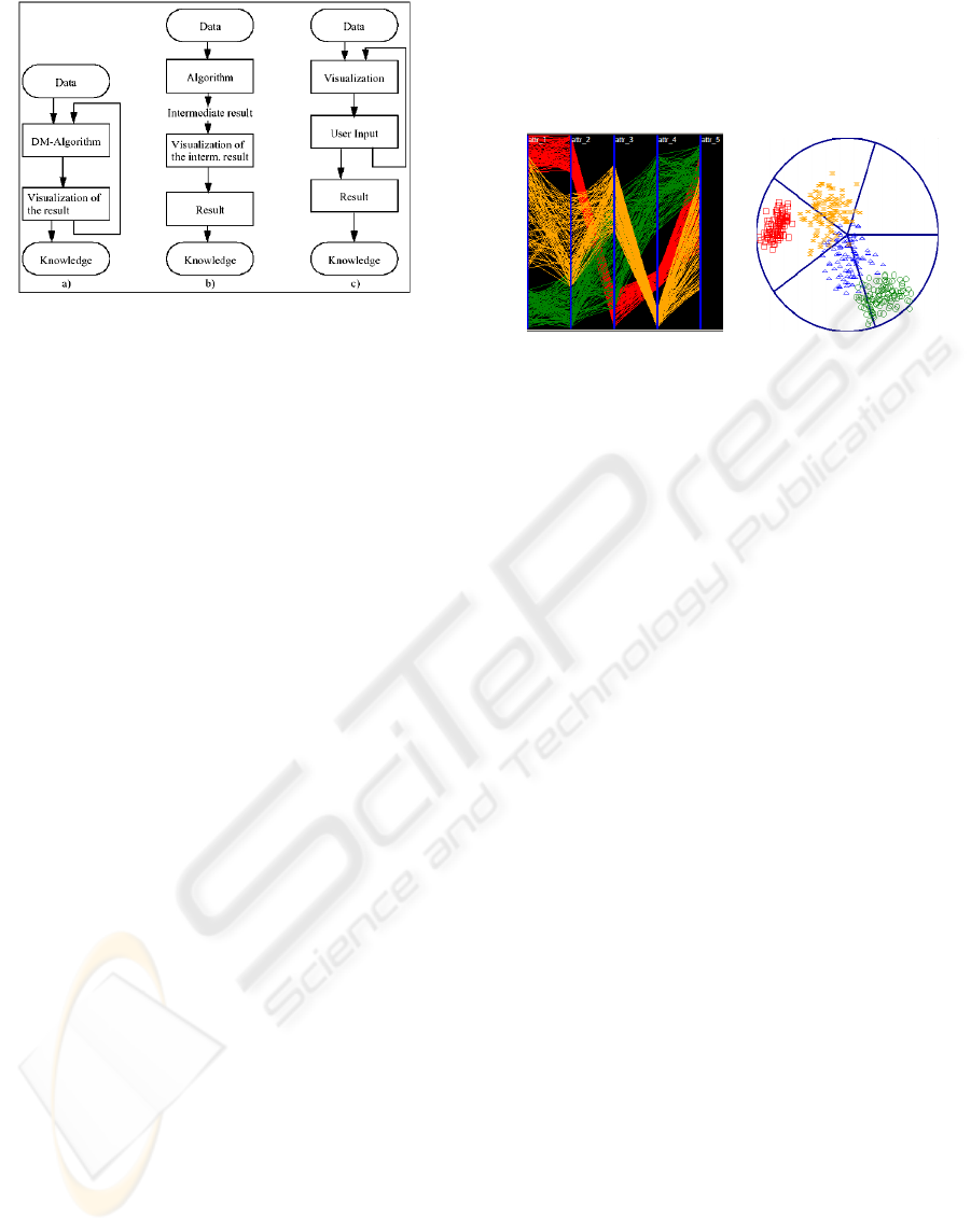
Figure 1: Architectures for Visual Data Mining.

Novel information visualization techniques have

been defined allowing a better exploration analysis

of large and multidimensional data sets. Most know

techniques are (Kantardzic, 2003): (i) Geometric

projection techniques. Projections for

multidimensional datasets; normally concerned with

the display of multidimensional spaces in a 2D

plane; (ii) Icon-based techniques. Display small

icons to represent attribute values; (iii) Pixel-

oriented techniques. Each object in the dataset is

represented by a pixel; and (iv) Hierarchical

techniques and graph. Information is displayed like

in a graph or hierarchy. Works like (keim 2002)

make an overview of these tecnhiques and tools.

Next we describe some visualization tools

related to this work. They are: (i) Parallel

Coordinate Plots (PCP) (Inselberg, 1985). The

objective is to represent a multivariable dataset in a

2D plane (like a screen of a computer). A backdrop

is drawn consisting of n equally spaced parallel lines

each one representing a dimension (figure 2.a)). For

each object a polyline is drawn and the position of

the vertex on the i-th axis corresponds to the i-th

coordinate of the object;

(ii) Radial Visualization (Hoffman, 1999). Its

goals are similar of PCP but the plane is represented

by a circle with axes equally spaced. The number of

axes is equall to the number of dimenions. An object

makes a physical strength in the i-th axe similar to

the i-th coordinate and a representative point is

drawn where the sum of all forces is zero (figure

2.b)). This tool enables an analysis of the efforts

made by dimensions. It is also a way to visually

display the structure or geometry of clusters; (iii)

Self Organized Maps (SOM) (Kohonen, 1990)

produces low dimension representation of training

samples while preserving the topological properties

of the input space. Useful to visualize, in a low

dimensional space, high dimensional data. It consists

in two steps. First a traning stage is made to build

the map with samples. Then a mapping stage is

performed to classify the input data. Each object is

represented by a vector with values from

dimensions. The object is associated to the cell with

the most similar vector

a)Parallel Coordinate Plot b) Radial Visualization

Figure 2: Example of geometric techniques.

2.3 Related Work

In (Nam, Han, Mueller, Zelenyuk, & Imre, 2007) a

visual tool, called cluster sculptor, is presented for

exploring large and high dimensional datasets. The

clustering engine implements a k-means algorithm.

Users are allowed to tune parameters interactively,

like: geometry, composition and spatial relations.

Their environment has tools for visually explore

hierarchical classifications by means of an

interactive dendrograma (operations like zoom,

merge and moving object between clusters).

In (Guo, Gahegan, MacEachren, & Zhou, 2005)

an integration of computational, visual and

cartographic methods is studied in order to visualize

multivariable spatial patterns. SOM is coupled with

a colour scheme to summarize a large amount of

data. Other novel visual data mining tool is PCP:

used to help interpreting multivariable patterns.

In (Demsar, 2006) investigates if combining

automated and visual data mining is suitable

approach for exploring geospatial data. The work

proves that novel visual elements, like snowflake

graphs, and SOM can be integrated with automatic

data mining algorithms like helping experts

investigate geodatasets.

In (Guo, Chen, MacEachren, & Liao, 2006)

present a novel geo-visual analytical strategy for

exploring and understanding spatial-temporal and

multivariable patterns. They also develop a

methodology to cluster, sort, and visualize large

datasets with spatial data allowing experts to

investigate large and complex patterns in spatial and

temporal dimensions.

SEMI-AUTOMATIC PARTITIONING BY VISUAL SNAPSHOPTS

3 A MODEL FOR VISUAL AND

SPATIAL CLUSTERING

As already stated, in a spatial cluster there are

objects with both semantic and spatial attributes; it

means, that clustering can be applied in

miscellaneous approaches. We propose the

following approaches, to get spatial clusters: (i) non-

spatial oriented. Apply the algorithm only to

semantic attributes. The spatial attribute is displayed

in a thematic map (spatial object, of the same

cluster, are drawn with the same color). This

spatiality of clusters enables the identification of

regions with similar behaviors. Inside a spatial

cluster, objects can be near, spread all over the space

or have some pattern correlated with some

relationship with another geographic phenomenon;

(ii) spatial and semantic oriented. Apply

algorithms both to semantic and spatial attributes

(separately). A thematic map is generated with two

different iconographic elements: one for semantic

patterns and other with a spatial pattern; (iii) spatial

oriented. Apply the algorithm to the spatial

attribute. For instance, identify the most central

entities of a layer (e.g., in a large area, where are

urban centres?); and (iv) multi-spatial oriented.

Apply algorithms to different layers tracking spatial

relationships, like topology, distance and directions.

This approach avoids pre-processing relations

between layers, making it possible to parameterize

spatial relations on-the-fly.

In this work, we use the non-spatial oriented

approach, and implement a visual data mining

architecture based on the visualization of

intermediate results (as presented in figure 1.b). .

In the context, of intermediate results

visualization, we formulate the following questions:

What is a stopping condition? How to handle more

than one stopping condition? When visualization

should be persecuted? What visual elements should

be used? Which actions should be allowed?.

We make the following considerations: First

experts are responsible for specifying relevant stop

condition, since they have more experience and

intuition about datasets; Second there must be some

flexible but controlled form to specify those

stopping stages, protecting the automatic process

against meaningless setting; Third in algorithms an

unit of work should be enclosed, to watch and check

his state; Fourth, since there are a large numbers of

dimensions and objects users can configure many

stopping condition.

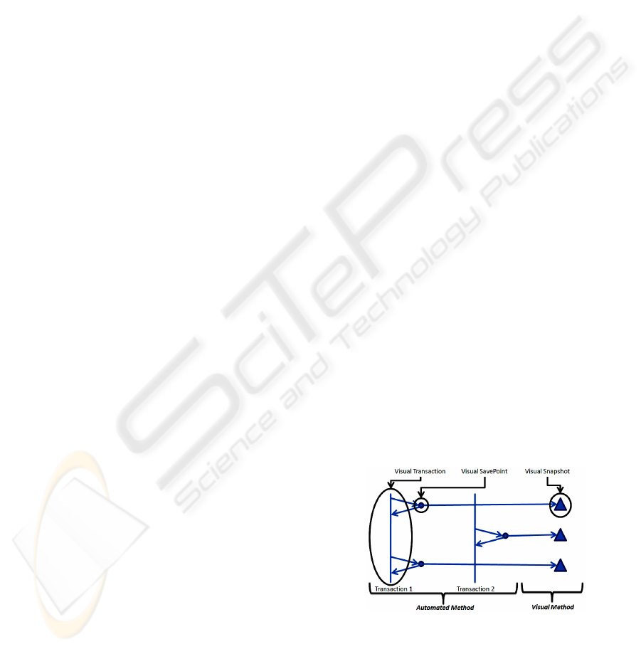
Next we make some definitions about concepts

for a spatial and visual data mining system. We call

the visual data mining workflow.

3.1 Visual Data Mining Workflow

In a semi-automated method a visual data mining

workflow is a group of visual data mining

transactions (one for every stop condition). A save

point detect a stop condition whose state can be

displayed through a visual snapshot. Next we make a

detail explanation of those concepts.

Definition 1. Unit of work. In medoid oriented

algorithms, a step is a unit of work that ends with

clustering (group of clusters) and has a timestamp.

The clustering state is measured computing: (i)

inter-cluster and intra-cluster similarities, for

instance, the number of objects, min, max and

average distance, distance between medoids,

cohesion and separation; (ii) is_link_pattern.

Intermediate patterns about values in dimensions

considerer relevant.

Definition 2. Visual save point. Happen when a

clustering has a state in agreement with a stop

condition, parameterized by experts. The automatic

method stops and gives rise to the visual method,

expressing the status of the current clustering.

Definition 3. Visual and spatial snapshot.

Graphic elements that express the state of a visual

save point and enables some level of interaction.

Definition 4. Visual data mining transaction. A

relevant condition. In the context of a visual data

mining workflow experts can configure many visual

data mining transactions (conditions). No meanwhile

the can be none or many save points.

Figure 3 shows the concepts associated to the

visual data mining workflow. The automated method

is coupled with the visual method.

Figure 3: Visual Data Mining Workflow.

How to stop the automatic method? We propose

three main parameterizations: (i) Using ‘must link’.

Subdivide into: Stop using semantic states – some

combination of values in a sub group of attributes;

ICEIS 2008 - International Conference on Enterprise Information Systems

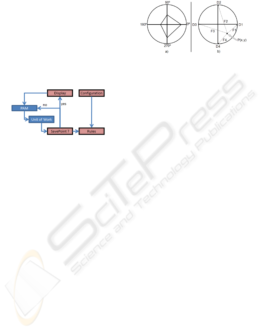
Stop using spatial states – geographic objects can

have specific relationships with other geographic

layers. For instance, in urban crime experts can

declare that violent crimes happen near old buildings

(the system looks to the relationship, in each cluster,

between the location of crimes and old buildings);

(ii) stop with periodicity. Use a regular step

interval; and (iii) stop using similarities between

steps. Verify if a constant metric is present between

clustering (from step to step) – if so maybe a cluster

has already been found.

Figure 4 presents a diagram showing the

interaction between automated and visual methods.

Figure 4: Stopping the process.

3.2 Exploring Clusters

An abstraction of a cluster is made using an ellipse,

whose size, colour and position are in agreement

with properties of clusters. A thematic map is

generated by cluster (each cluster has a different

colour). If the dataset is large, instead of displaying

geographic objects, a geometric approximation can

be computed, for each cluster, allowing a more

suitable observation.

The visual elements for exploring clusters are: (i)

Cluster Abstraction. A group of ellipses represents

a group of clusters; (ii) Interactive PCP.

Understand the data distribution inside and between

clusters; and (iii) Interactive RV. Understand data

distribution and structure inside and between

clusters.

The interaction model has synchronized

granularity managed and controlled by a central

component (controls the parameterization of colours

and the display of clusters and attributes).

3.2.1 Visual Abstraction of Clusters

The ellipse is rendered on screen on a position

computed by the spring model stated in section 2.2.

The spring model enables the computation of central

points in screen using values of medoids. Figure 5a)

shows an ellipse where the number of axes is equal

to the number of attributes (four). In each axe the

strength is equal to the attribute value. Figure 5b)

shows the equilibrium point (central point).

Figure 5: Computing the screen central point of a cluster

using the medoid.

In equation 1, α represents an angle, β is the

angle step and

d is the value made, at α, by a

dimension d.

3.2.2 Interactive PCP

PCP is a component that projects the spectrum of

clusters through dimensions translating an n

dimension space in a 2D space. Using a colour

scheme is possible to distinguish clusters from each

other. By observing the map and the PCP users have

a legend for interpreting the projection of

dimensions in the map (Guo, Gahegan, MacEachren

& Zhou (2005)). No meanwhile, more can be done.

In this work, interactive exploration is improved by

allowing: (i) attribute reorder. The expert sets

relevant attributes side by side in order to compare

them and conclude, for instance, that in a cluster the

combination of some attribute values are correct; (ii)

attribute zooming. The expert makes a closer look

at some detail in a dimension in order to better

understand how values spread over the dimension. If

all clusters have a similar value in a dimension then

users can conclude that the dimension doesn’t have a

strong influence in the identification of clusters and

so can be removed in a subsequent step; (iii)

attribute hide. Similar to reorder but dimension

disappear from the component; (iv) cluster cut.

Turning clusters visible or invisible allowing a better

observation of one or some clusters; and (v)

attribute move. Automatic had-doc position

ordering by exchanging plane positions allowing the

observation of all possible combinations in

dimensions; (vi) store the picture. In a black box

execution, the current projection of clusters in PCP,

can be stored as an image in disk enabling a future

analysis; (vii) values cut. Using the mouse users can

draw a rectangle in order to watch, in the PCP, only

objects whose values are inside some selected area

excluding values that are not interesting; change

⎪

⎩

⎪

⎨

⎧

×=

⇔=

∑

º360

)(

)cos(

βαα

αω

dseny

(1)

SEMI-AUTOMATIC PARTITIONING BY VISUAL SNAPSHOPTS

layout. Experts can make a new thematic

parameterization of clusters changing colors, size of

lines.

3.2.3 Interactive RV

Interactive RV also projects an n dimensional space

in a 2D space. In this case, dimensions are axes of an

ellipse making it possible to observe the

combination of strengths made by dimensions

(higher or lower values). It uses colors and icons to

render clusters.

This component has the same operations with the

same meaning retracted in Interactive PVP, namely:

(i) attribute reorder; (ii) attribute zooming; (iii)

attribute hide; (iv) cluster cut; (v) attribute move;

(vi) store the picture; and (vii) values cut; (vii)

change the layout.

The image produced by this component makes it

possible to analyze the spatial structure of clusters in

a 2D space. Tracking intermediate stages by storing

images produced by this component enables a dipper

comprehension about how clusters are formed along

the time.

All actions in RV also have impact in the map and

the PCP. Also in the map an operation (topology,

distance, and direction) restricts the data that is

displayed in others components.

4 CASE OF STUDY:

ANALYSING AN URBAN

INFRASTRUCTURE

In order to identify the benefits of the described

concepts, a scenario related to an urban drainage

infrastructure, implemented in small urban areas, is

used for experiments. Users are allowed to identify

correlations inside a spatial cluster and between

spatial clusters. The approach is non-spatial

oriented. The spatial dataset has a geographic

attribute representing pieces of the network having

each the following semantic attributes:

Year: (<1975, [1980-1985], 1[987-1994], >1994).

Status: A classification of the actual situation of a

chunk (active, proposed, future).

Station: A classification of the type of station for

residual water treatment (ETAR, FOSSA)

Material: (Material, Class). A classification of

material used to build the network (GRES, PVC,

PVCC).

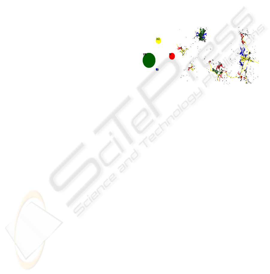
The algorithm PAM was changed stopping at

configured save points and displaying intermediate

results. The dataset has 400 objects and 4

dimensions. Results for four clusters are presented.

Figure 6 shows an image with spatial clusters

obtained after the application of the automatic

method. The size of ellipses expresses the amount of

objects allocated to clusters. In thematic maps, the

color used to paint a geographic object identifies his

cluster. In the ellipse a label identifies her medoid.

Figure 6: Visualization of spatial clusters.

The green cluster (115) is the largest, being their

spatial component concentrate in two areas; after

overlapping the map with a layer of buildings, it can

be pointed out that geographic objects are

concentrated in the middle of urban areas. The red

cluster (91) is located at non-dense regions (rural

regions). The yellow (302) cluster is associated to

the highest networks (the ones that are connecting

small rural regions). Finally, the blue cluster (91)

takes place in low concentrated regions.

After this visual interpretation, a closer look to

semantic attributes can be persecuted allowing the

interpretation of the semantic and spatial

correlations.

In figure 7 the interactive PCP and interactive RV

are displaying attributes and dimensions to users;

through a set of checkboxes is possible to execute on

the fly combinations of clusters with dimensions.

The image figure 7.a) shows that objects have very

similar values at adjacent dimensions like

tmanutencao and tmaterial since lines that connect

them are overlapped (yellow lines belong to the last

rendered cluster). This can have two meaning: (i)

dimensions do not contribute to cluster formation; or

(ii) small differences can be a factor to a cluster

formation if the others dimensions are more similar.

ICEIS 2008 - International Conference on Enterprise Information Systems

In figure7.b) RV confirms object similarity in the

two dimensions by showing that the distribution of

objects along those two dimensions is concentrated.

Figure 7: Interactive PCP and Interactive RV.

In figure 8 sample images of interactive PCP are

presented.

a) b)

Figure 8: Visual combining of attributes.

The user performs a cluster cut selecting only the

two largest clusters (green and red), in order to

comprehend then. Then it performs attribute hide

in order to analyze the behaviour of the dimension

labeled tano. It can be pointed that the two clusters

have more similarities between labeled dimensions

tano and ttratamento (figure 8.a)).

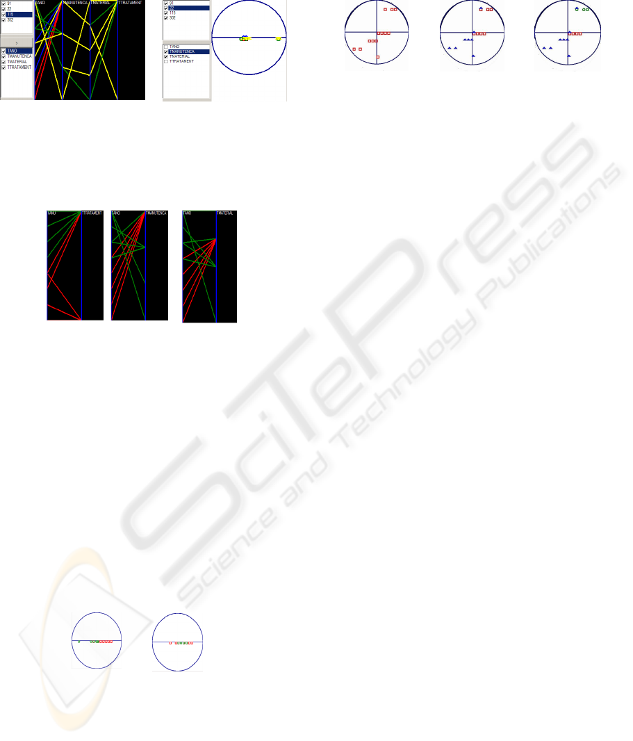
Users can be confused about which pair of attributes

are more similar: (tano, tmanutencao) or (tano,

tmaterial). Using RV with only those dimensions

users can, for instance, conclude that the pair

(tano,tmaterial) is more dissimilar than (tano,

ttratamento) since, in the first pair, objects are

more spread over dimensions (figure 9).

Figure 9: Using the interactive RV to visually discover

similarities in dimension.

Figure 10 shows images about visual save points

related to a visual data mining transaction. It is

possible to observe the evolution of the clustering

process along the time and make some conclusions.

For instance, between save points 2 and 3 the

structure of a cluster (blue triangles) is maintained

which can mean that a cluster match has been

reached.

a) SavePoint 1

b) SavePoint 2

c) SavePoint 3

Figure 10: The evolution of a clustering process displayed

in RV and stored in disk.

In a large dataset, the process could be improved if a

prior cluster is found. Users are allowed to stop the

current automatic method and start it with a lower

number of objects, by eliminating the ones that

belongs to a validated cluster (data reduction) or

eliminating dimensions that do not make a strong

contribution to cluster discovery (dimension

reduction).

In a large dataset, experts can stop the current

automatic method and start it with a lower number

of objects, eliminating the ones that belong to valid

clusters already discovery.

5 CONCLUSIONS AND FUTURE

WORK

In this work a visual data mining system is presented

allowing some degree of interaction with

intermediate stages of automatic methods. The

concept of spatial data mining transaction is defined

has a group of visual save points that are in

agreement with a user stop condition. In a visual

save point a visual snapshot is generated showing

result of intermediate steps. In it experts can

conclude that a cluster as been found by exploring

attribute values combination. For that visual data

mining tools like PCP and RV are implement with

new operations allowing better attribute exploration

(like reorder, zooming, hide). Future work will be

done at the automatic method level by trying to

improve the interaction with clustering enabling a

more suitable way of attribute and data reduction.

REFERENCES

Ankerst, M. (2000). Visual Data Mining (PhD Thesis).

Munich: Institute of Computer Science, University of

Munich.

a) Interactive PCP (all

dimensions and attributes)

b) Interactive RV (only

some dimensions)

SEMI-AUTOMATIC PARTITIONING BY VISUAL SNAPSHOPTS

Demsar, U. (2006). Data Mining of Geospatial Data:

Combining Visual and Automatic Methods.

Stockholm: Royal Institute of Technology (KTH).

desJardins, M., MacGlashan, J., & Ferraioli, J. (2007 ).

Interactive Visual Clustering. Proceedings of the 12th

international conference on Intelligent user interfaces

(pp. 361 - 364 ). Honolulu, Hawaii, USA : ACM Press

Gahegan, M., & Brodaric, B. (2002). Computational and

Visual Support for Geographical Knowledge

Construction: Filling in the gaps between exploration

and explanation. Advances in Spatial Data Handling,

Proceedings of the 10th International Symposium on

Spatial Data Handling.

Guo, D., Chen, J., MacEachren, A. M., & Liao, K. (2006).

A Visual Inquiry System for Space-Time and

Multivariable Patterns (VIS-STAMP). Transactions on

Visualization and Computer Graphics , 12 (6), 1461-

1474.

Guo, D., Gahegan, M., MacEachren, A. M., & Zhou, B.

(2005). Multivariate Analysis and Geovisualization

with Integrated Geographic Knowledge Discovery

Approach. Cartography and Geographic Information

Science , 32 (2), 113-132.

Guo, D., Peuquet, D. J., & Gahegan, M. (2003). ICEAGE:

Interactive Clustering and Exploration of Large and

High-Dimensional Geodata. GeoInformatica (pp. 229-

253). The Nertherlands: Kluwer Academic Publishers.

Hoffman, P. (1999). Table Visualization: A Formal Model

and Its Applications (PhD Thesis). Lowell LA, USA:

University of Massachusetts Lowell.

Ibrahim, L. F. (2005). Using Clustering Algorithm CWSP-

PAM for Rural Network Planning. Third International

Conference on Information Technology and

Applications (ICITA'05) (pp. 280-283). Sydney: IEEE

Computer Society.

Imrich, P., Mueller, K., Mugno, R., Imre, D., Zelenyuk,

A., & Zhu, W. (2002). interactive Poster:Visual Data

Mining with the Interactive Dendogram. Information

Visualization Symposium.

Inselberg, A. (1985). The plane with parallel coordinates.

Visual Computer , 1 (4), 69-81.

Jiang, B. (2004). Spatial Clustering for Mining Knowledge

in Support of Generalization Process in GIS. ICA

Workshop on Generalisation and Multiple

Representation. Leicester, United Kingdom.

Kaufman, L., & Rousseeuw, P. (1990). Finding Groups in

Data: An Introduction to Cluster Analysis. John Wiley

& Sons.

Kantardzic, M. (2003). Data Mining: Concepts, Models,

Methods, and Algorithms. Danvers, MA, USA: John

Wiley & Sons.

Keim, D. A. (2002). Information Visualization and Visual

Data Mining. IEEE Transactions on Visualization and

Computer Graphics , 100-1007.

Kriegel, H.-P., Kunath, P., Pfeifle, M., & Renz, M. (2006).

ViEWNet: Visual Exploration of Region-Wide Traffic

Networks. Data Engineering, 2006. ICDE '06.

Proceedings of the 22nd International Conference on

(pp. 166-166). Atlanta, USA: IEEE Computer Society.

Koua, E. L., MacEachren, A., & Kraak, M.-J. (2006).

Evaluting the usability of visualization methods in an

exploratory geovisualization environment.

International Journal of Geographical Information

Science , 20 (4), 425-448.

Liu, W., Seto, K. C., & Sun, Z. (2005). Urbanization

Prediction with ART-MMAP Neural Network Based

Spatial-Temporal Data Mining Method. 5th

International Symposium Remote Sensing of Urban

Area (URS 2005), XXXVI. Tempe, AZ, USA.

May, M., & Savinov, A. (2004). SPIN! AN ENTERPRISE

ARCHITECTURE FOR DATA MINING AND

VISUAL ANALYSIS OF SPATIAL DATA. In B.

Kovalerchuk, & J. Schwing, Visual and Spatial

Analysis (pp. 293-317). Dordrecht, The Nertherlands:

Springer.

Nam, E. J., Han, Y., Mueller, K., Zelenyuk, A., & Imre, D.

(2007). ClusterScultor: A Visual analytics Tool for

High-Dimensional Data. IEEE Symposium on Visual

Analytics Science and Technology 2007 . Sacramento,

CA.

Ng, R. T., & Han, J. (2002). CLARANS: A Method for

Clustering Objects for Spatial Data Mining. IEEE

Transaction on Knowledge and Data Enginnering , 14

(5), 1003-1016.

Ng, R. T., & Han, J. (1994). Efficient and Effective

Clustering Methods for Spatial Data Mining. 20th

VLDB Conference. Santiago, Chile.

Schulz, H.-J., Nocke, T., & Schumann, H. (2006). A

Framework of Visual Data Mining of Structures. 29th

Australasian Computer Science Conference (pp. 157-

166). Hobart, Australia: Australian Computer Society,

Inc.

Tung, A. K., Hou, J., & Han, J. (2001). Spatial Clustering

in the Presence of Obstacles. 17th International

Conference on Data Engineering (ICDE'01).

washington, DC, USA: IEEE Computer Society.

Torun, A., & Duzgun, S. (2006). Using Spatial Data

Mining Techniques to Reveal Vulnerability of People

and Places Due to Oil Transportation and Accidents: A

Case Study of Istanbul Strait. Proceedings of the

ISPRS Vienna 2006 Symposium, (pp. 43-48). Vienna.

Wan, L.-H., Li, Y.-J., Liu, W.-Y., & Zhang, D.-Y. (2005).

Application and Study of Spatial Cluster and

Customer Partitioning. Fourth International

Conference on Machine Learning and Cybernetics (pp.

1701-1706). Guangzhou: IEEE.

Wang, X., & Hamilton, H. (2005). Clustering Spatial Data

in the Presence of Obstacles. International Journal on

Artificial Intelligence , 14, 177-198.

Zhang, X., Wang, J., & Wu, F. (2006). Spatial Clustering

with Obstacles Constraints Based on Genetic

Algorithms and K-Medoid. IJCSNS International

Journal of Computer Science and Network Security , 6

(10), 109-114.

ICEIS 2008 - International Conference on Enterprise Information Systems