
Transient IC Engine Monitoring Under Temperature
Changes Using an AANN
Xun Wang
1
, George W. Irwin
1
, Geoff McCullough
2
, Neil McCullough
2
and Uwe Kruger
3
1
Intelligent Systems and Control Research Group, Queen’s University Belfast BT9 5AH, U.K.
2
Internal Combustion Engines Research Group, Queen’s University Belfast BT9 5AH, U.K.
3
Department of Electrical Engineering
The Petroleum Institute, PO Box 2533, Abu Dhabi, U.A.E.
Abstract. This paper reports on non-linear principal component analysis for
fault detection on an internal combustion (IC) engine. An auto-associative
neural network (AANN) model is built from transient engine data collected
under varying atmospheric conditions. The experimental data used for
modelling was collected for two different drive cycles, the Identification Cycle
and the New European Drive Cycle. The key issue here is to decide which data
should be used for training the neural network to produce good fault detection
generalisation under different atmospheric conditions and with a different drive
cycle. This is achieved successfully, with the Q monitoring statistic indicating
an absence of unwanted false alarms under fault-free operation, along with
successful detection of air leaks of varying magnitude in the inlet manifold.
1 Introduction
The specific provisions of more general emissions legislation relating to the detection
of faults within an internal combustion engine is commonly known as On-Board
Diagnostics (OBD). This details both the component parts of the engine to be tested
and at what frequency. This monitoring entails the diagnosis of any fault, which could
cause the tailpipe emissions of carbon monoxide (CO), unburned hydrocarbons (HC)
and oxides of nitrogen (NO
x
) to rise above legislated values.
The automotive industry currently employs a combination of signal and model-
based diagnostic techniques for OBD, the latter being based mainly on physical
models of the system. However, as the emissions thresholds have reduced in response
to increasingly stringent regulation demands, the OBD fault detection thresholds have
tightened accordingly, thereby increasing the challenge in engine modelling and
monitoring (Stobart, 2003) with over 50% of engine control unit software being
currently devoted to OBD. The complexity of physical models will have to increase
dramatically if the smaller variations in emissions, constituting a fault under future
OBD regulations are to be successfully detected. Further, such models will require
extensive on-line validation for each engine and vehicle derivative. Consequently, the
cost of developing and validating physical models will increase exponentially. Over
Wang X., W. Irwin G., McCullough G., McCullough N. and Kruger U. (2008).
Transient IC Engine Monitoring Under Temperature Changes Using an AANN.
In Proceedings of the 4th International Workshop on Artificial Neural Networks and Intelligent Information Processing, pages 28-40
DOI: 10.5220/0001507900280040
Copyright
c
SciTePress

the last decade the mathematical complexity and computational intensity of physical
model-based OBD has stimulated research on alternative fault detection and diagnosis
approaches suitable for automotive engines (Nyberg, 1999; Grimaldi et al., 2001;
Crossman et al., 2003; Kimmich et al., 2005.)
Some work has also been done on statistical methods, including principal
component analysis (PCA) where a reduced set of statistically independent score
variables are generated for process monitoring. Unfortunately, while PCA in its
original form is only applicable to linear data, a nonlinear extension in the form of an
auto-associative neural network (AANN) (Kramer, 1992) is now available, where the
scores are produced in the network bottleneck layer. Because of its conceptual
simplicity and close relation to linear PCA, our previous work on diesel engines used
an AANN for monitoring during steady-state operation (Antory et al., 2005),
including increased sensitivity in detecting minor faults (Wang et al., 2008a) by
incorporating additional analysis in the form of the statistical Local Approach.
Nonlinear PCA (NLPCA) has also proved to be effective when applied to
experimental data recorded from the air intake system of a gasoline engine during
transient operation (Wang et al., 2008b). Here the AANN was trained on a modified
identification (MI) cycle, specially designed to ensure that the engine speed and
throttle position covered the complete operating map at rates similar to those
experienced during normal operation. Importantly, the resulting model proved
suitable for more general use with the New European Drive Cycle (NEDC), a
standardised test for all new model types representing a mixture of urban and
motorway driving. In this work also, rather than using the same operational cycle for
AANN training and testing, two completely different engine drive cycles will be
employed, as detailed later.
The major limitation in all the previous work is the absence of any consideration of
the effects of atmospheric changes on the ability of the model-based fault detection to
generalise in terms of avoiding false alarms while correctly identifying fault
conditions. Thus, the experimental data used for validating the AANN model and the
faulty data sets were all recorded under similar atmospheric temperature and pressure
conditions to those for the training data. Moreover, none of the measured engine
variables previously included in the monitoring model was in fact significantly
affected by such atmospheric changes. Any AANN model derived for IC engine
monitoring under laboratory conditions, should also be capable of being generalised
to a wider range of driving conditions. The aim of the present paper is to address this
important deficiency. The practical significance of the results reported later is that the
experimental data sets available for neural modelling not only covered two different
operational cycles, as required for dynamic monitoring, but were also recorded under
different temperature conditions.
Some work on the effect of changes in atmospheric pressure and temperature on
the performance of an engine has been reported in the literature, but from the
perspective of engine design (Sher, 1984). Here computer code was developed to
simulate the engine cycle for the purpose of evaluating an optimal engine design
giving the best performance at high altitude conditions. The focus of this paper is data
modelling of a modern automotive petrol engine, based on which its fault monitoring
under different driving conditions can be achieved. This further significantly extends
29
the generalisation abilities of the AANN IC engine model described in our previous
work.
The paper is organised as follows. An introduction to the experimental petrol IC
engine facility, the engine drive cycles and the data collection regime is given next in
Section 2. Following a brief review of NLPCA, Section 3 then presents the
experimental condition monitoring results. The paper ends with a brief discussion,
some conclusions and suggestions for future research.
2 Automotive Engine Tests
This section briefly describes the experimental engine test-bed, followed by detailed
explanations of the data collection regime under both normal and faulty operating
conditions.
2.1 Engine Test Cell
The target application was a four-cylinder 1.8 litre spark ignition engine,
manufactured by Nissan. This engine represents current technology with devices such
as variable valve timing, inlet swirl plates, exhaust gas recirculation and a close-
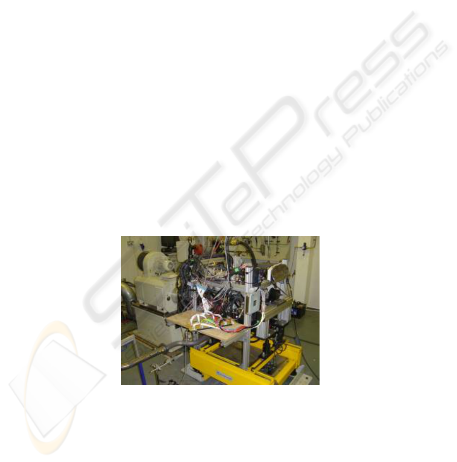
coupled catalyst. The engine installation can be seen in .
The engine was installed in a state-of-the-art test facility at Queen's University
Belfast. An AC dynamometer with a Ricardo S3000 controller was used to control the
engine throughout the simulated transient drive cycles. Sensor signals were recorded
using the testcell data acquisition hardware – a Ricardo TaskMaster 500/2000 system,
capable of recording up to 32 analogue input channels simultaneously.
Fig. 1. View of engine test-bed and dynamometer.
The intake subsystem of this engine was investigated. In order to simplify the air
intake modelling, the exhaust gas recirculation (EGR) function was disabled. The
following five variables were used to analyse this subsystem: crankshaft rotational
speed (rev/min), pedal position (%), mass air flow (kg/h), inlet manifold pressure
30

(bar) and inlet manifold temperature (ºC). Rotational speed and pedal position formed
the engine inputs, while the other variables represented the dynamic behaviour of the
intake system. Importantly, these variables are all available from current sensors fitted
to the standard vehicle and so the modelling and fault detection system for OBD
outlined in this paper requires no additional hardware.
In contrast to our previous work on this IC engine where atmospheric conditions
were not considered, it will be seen that including the inlet manifold temperature in
the data modelling allows atmospheric temperature changes to be incorporated, as
shown later in subsection 2.3.
2.2 Atmospheric Changes
The atmospheric temperature and pressure both affect the dynamic performance of an
IC engine and so must be accounted for in any model-based OBD scheme. This study
is confined to consideration of the variation in atmospheric temperature, since
atmospheric pressure control in the engine test cell was not available.
The experimental engine data sets were collected at two different temperature
conditions. Normal room temperature (RM) was around 20-25ºC and required no
manual intervention. The elevated temperature (ET) condition was controlled at 30-35
ºC by electrical heating of the combustion air. The engine’s performance under these
two temperature conditions is analysed below, after the two drive cycles have been
introduced.
2.3 Drive Cycles
The New European Drive Cycle (NEDC) is used for emissions certification of light
duty vehicles in Europe. It is composed of various sections which simulate both urban
and motorway driving conditions. The measurement of the resulting exhaust
emissions forms one component of the Type Approval test, which is compulsory for
any new vehicle model entering the European market. Alternative drive cycles
include the FTP 75 used in the USA and the 10-15 Mode Cycle adopted by Japan.
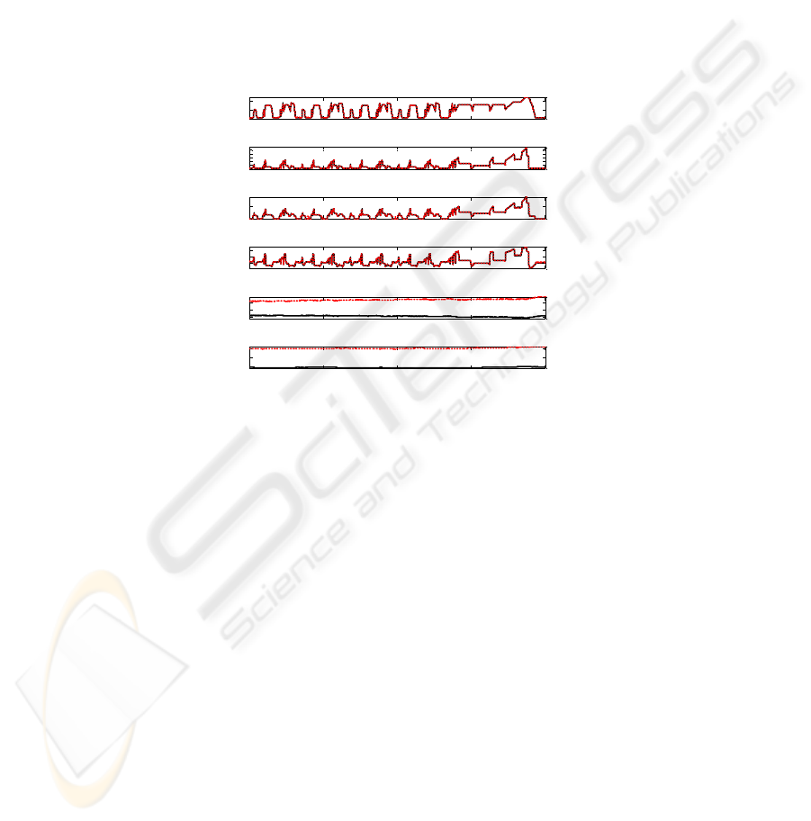
The variation in the engine speed and pedal position inputs produced by the NEDC
for a sampling rate of 10Hz are shown in the top two plots of Fig. 2. Note that Fig. 2
shows two experimental data sets, corresponding to the RM (black) and ET (red)
temperature conditions respectively. In addition to the five engine variables, the figure
also includes the atmospheric temperature. The reason for including the atmospheric
temperature is to help visualise the impact of its change on the engine performance.
This variable is not to be included in the subsequent engine modelling.
It is clear from Fig. 2 that the NEDC is a highly transient cycle which includes
periods of rapidly varying engine speed and pedal position inputs as gear changes are
simulated. During vehicle deceleration, when the pedal position is zero, the engine
speed is often higher than idle speed. Here the engine is motored through the
transmission which contributes to the vehicle’s braking requirement. These phases of
the NEDC were simulated during testing by supplying a torque input from the
motoring dynamometer to maintain the commanded engine speed.
31
In the example shown in Figure 2, the temperature of the air drawn into the intake
manifold in the RM case is increased slightly above the atmospheric temperature due
to heat transfer from the warm engine. The average inlet manifold temperature is
therefore around 26
o
C. Conversely, in the ET case, the temperature of the air supplied
to the engine is higher than that of surrounding environment and so some heat is lost
by convection from the intake manifold, reducing its temperature to around 32
o
C on
average. Assuming the volumetric efficiency of the engine remains the same for a
given combination of inputs, the increase in temperature between the RM and ET
cases reduces the density of the air, and hence the mass air flow rate, entering the
engine by around 2%. The intake manifold pressure was unaffected by the change in
atmospheric temperature.
1000
3000
Engine Speed (rpm)
5
25
Pedal Position (%)
0
20
Mass Air Flow (g/sec)
0.4
0.8
Intake Manifold Pressure (bar)
26
30
Intake Manifold Temperature (ºC)
5 10 15 20
25
35
Atmospheric Temperature (ºC)
Time (min)
Fig. 2. Engine variables for the NEDC (10Hz sampling) with RM (black) and ET (red)
atmospheric temperatures.
While the NEDC is indeed a highly dynamic cycle, and is purported to be
representative of typical vehicle use,
Fig. 4 shows that the engine control inputs do not
cover the whole operational map. For example, engine speed does not exceed
3500rpm while the throttle pedal position is less than 15% for most of the cycle,
briefly reaching a maximum of around 28% at 3500rpm during the motorway driving
phase. This represents only 55% of the peak torque available at that engine speed.
This analysis implies that data from the NEDC would be unsuitable for training an
AANN model. Inaccurate predictions would be produced and false alarms generated,
when the IC engine is operated outside the regions of the map accessed during
training.
An alternative drive cycle, the Kimmich identification cycle (KI cycle), was also
considered to provide better coverage of the operating region (Kimmich et al., 2005).
However, although this cycle indeed produces a broader range of engine speeds and
throttle positions, the rate at which these variables change is very significantly lower
than that experienced in real driving. The NEDC by contrast is more dynamic in
nature and does produce more realistic transients. A modified identification (MI)
cycle was therefore designed to generate suitable data for transient modelling. This
32
was developed by examining the sections of the NEDC where the engine speed was
undergoing the greatest transients, which occurs during accelerations in 1st gear. The
timescale of the KI cycle was then reduced by a factor of 5.7 such that the rate of
change of engine speed matched that of the most transient section of the NEDC. The
resulting MI drive cycle therefore combines the benefits of both the KI one and the
NEDC as it produces good coverage of the engine operating map, while also
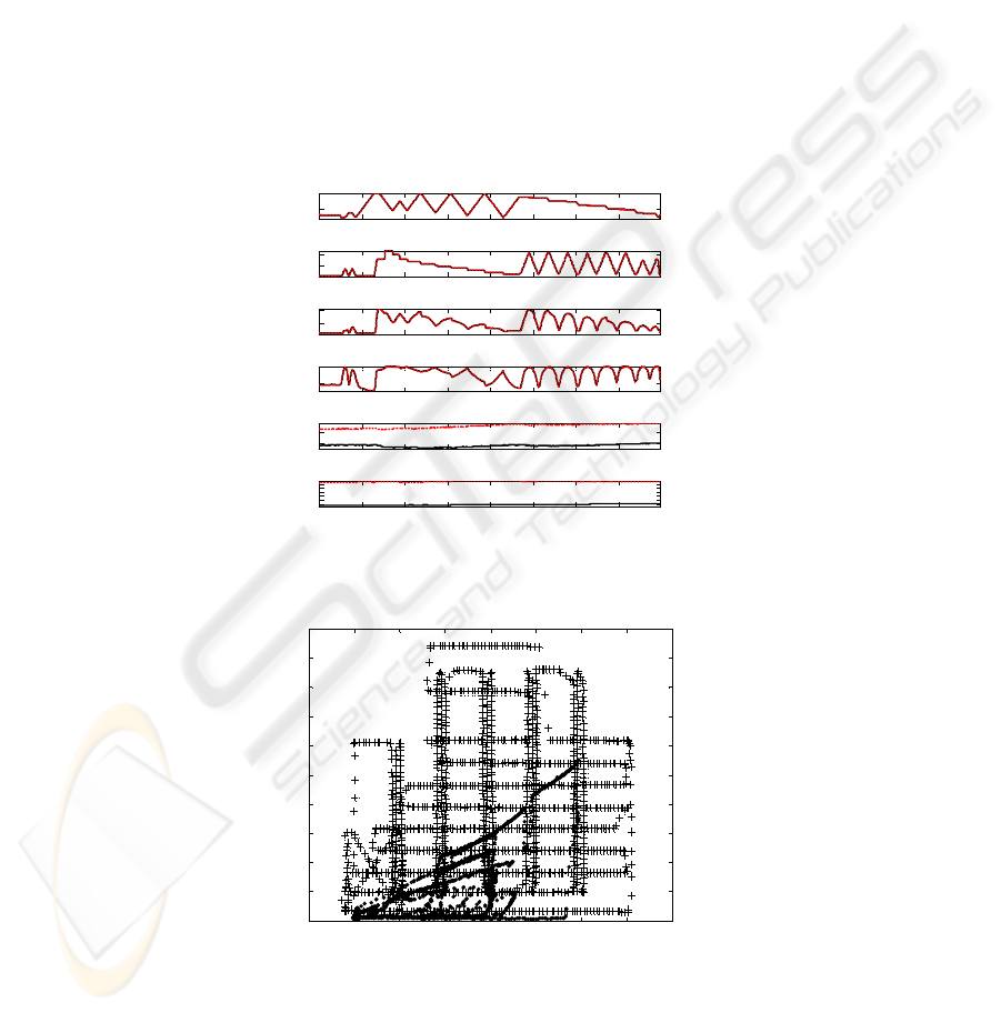
simulating realistic dynamics. The engine inputs for the MI cycle and corresponding
outputs for the same two cell temperature conditions as before are shown in Figure 3.
The same observation can be made as for the NEDC responses in Fig. 2 viz. that only
the inlet manifold temperature has been affected by the atmospheric temperature
change.
Comparing the operating maps of the MI and NEDC cycles in
Fig. 4, it is clear that
any model built on engine data from the former cycle will better represent a much
wider range of IC engine operation, as required.
2000
4000
Engine Speed (rpm)
20
40
Pedal Position (%)
20
40
Mass Air Flow (g/sec)
0.5
1
Intake Manifold Pressure (bar)
24
26
Intake Manifold Temperature (ºC)
1 2 3 4 5 6 7
22
32
Atmospheric Temperature (ºC)
Time (min)
Fig. 3. Engine variables for the modified identification (MI) cycle with RM (black) and ET
(red) atmospheric temperatures.
500 1000 1500 2000 2500 3000 3500 4000 4500
0
5
10
15
20
25
30
35
40
45
50
Engine Speed (rpm)
Throttle Position (%)
Fig. 4. Comparison of engine operating maps for the NEDC (circles) and MI (crosses) drive
cycles.
33

2.4 Data Collection
The MI cycle last about 8 minutes, providing 4785 data points. This cycle was
repeated three times for both RM and ET conditions without introducing any engine
fault. This generates two sets of engine data for model building, the third being
reserved to validate the model. A further single set of NEDC data was recorded
during normal ‘fault-free’ operation under both RM and ET conditions, in order to
assess the generalisation capability of the trained AANN model on unseen data.
2.5 Air Leak Fault
In this investigation, the faulty conditions took the form of air leaks of varying sizes
in the intake manifold. This is indicative of a process, rather than sensor fault, and is
representative of a leakage past a gasket or fitting between the throttle plate and the
intake valve. A minor air leak potentially may not be noticeable to the driver.
Nevertheless, when a fault of this type occurs, the driver would adjust the throttle
pedal until the desired torque is achieved. Thus, in this fault scenario it is imperative
to preserve the values of the engine speed and pedal position between the fault-free
and faulty conditions. The fault was introduced by drilling a hole into a bolt which
was then screwed into the inlet manifold of the engine downstream of the throttle
plate. A total of four such bolts were used: a solid one to produce the fault-free
condition, and three others with 2mm, 4mm, and 6mm diameter holes to introduce
faults of differing magnitude. Data representing all three faulty conditions were
collected for both the MI cycle and the NEDC.
3 Nonlinear PCA
The AANN shown in Fig. 5 is a special neural network architecture with 3 hidden
layers, referred to as the mapping, bottle-neck, and demapping layers respectively.
Fig. 5. Auto associative neural network architecture for nonlinear PCA.
The AANN represents an identity mapping for a given set of n variables, such that
the network inputs and outputs are identical. A hyperbolic tangent function was used
34

as the activation function in the mapping and de-mapping layers, while the other two
layers contained linear activation functions. Note also the presence of direct links
from the inputs to the bottleneck layer and from the bottleneck layer to the outputs.
This network is regarded as a nonlinear version of PCA because of its similarity in
producing ‘scores’, normally fewer in number than the original variables from a given
process. The scores generated by linear PCA are based on the linear relationships
among the physical variables, and can effectively represent the variance in these
variables. The scores can then be used for reconstructing the original variables or for
monitoring any unknown data from the same process. In the case of NLPCA, the
ni < nodes in the bottleneck layer represent the nonlinear scores,
i
tt ,,
1
"
. They
are obtained by capturing the nonlinear relationship between the engine variables in
the input layer. The scores are then able to reconstruct the original variables by
passing them through the de-mapping layer to the output layer. If only linear
relationships exist between the engine variables, the scores from such a NLPCA
model should in theory be the same as those from a PCA one.
The mathematical description of the identity mapping can be described in two
parts. The scores are produced in Figure 5 by the mapping layer that constitutes a
nonlinear transformation on the inputs. Thus, for the k
th
score:
)(xt
kk
G
=
(1)
The variables at the output layer
x
′
can then be obtained using:
(
)
T
ijj
tttHx "
21
=
′
(2)
The AANN network parameters are trained by minimising the cost function:
∑
=
′
−=
n
j
jj
xxJ
1
2
)(
(3)
When the NLPCA has been trained from fault-free data, a Q statistic can be
calculated based on the model prediction error as
ee
T
Q =
(4)
Here
e
refers to the difference between the model prediction vector and its
measured value for one sample. Q follows a central
2
χ
distribution and appropriate
confidence limits can be estimated as discussed in Jackson, 1991. The values of the Q
statistic from the training data were used to calculate 95% and 99% confidence limits,
which are subsequently used as benchmarks for monitoring unknown data from the
engine.
35

4 Results
Choosing the best training set from the fault-free MI cycle data sets to use for AANN
training required careful consideration. Three data sets had been generated for each of
the two atmospheric temperature conditions. Moreover, the atmospheric temperature
varied by 2 or 3 degrees during the three repetitions of the MI drive cycle. Although
minor, this variation will have an impact on the generalisation of any engine model.
The principle used in selecting training data here was to choose the fault-free data
with the widest possible range of temperature conditions, while leaving adequate
fault-free data for validation. Closer inspection showed that data sets one and three,
under either RM or ET temperature conditions, provided a much wider range of
temperature coverage than any alternative pairing. The training data used in this work
therefore consisted of four MI cycles corresponding to data sets one and three under
each of RM and ET temperature conditions. The second data sets, collected under
both RM and ET temperature conditions were then employed for validation purposes.
Subsection 4.1 provides details of how the model was trained, along with its
validation on the MI cycle. The generalisation capability of the resulting engine
model is assessed in section 4.2, while its ability to detect air leak faults with the
engine operating under both the MI and NEDC cycles is presented in subsections 4.3
and 4.4 respectively.
4.1 Training and Validation
The NLPCA built on the training data had a 5-10-4-10-5 structure, with 10 nodes in
the mapping and de-mapping layers and 4 in the bottle-neck layer. Having trained the
model it was subsequently validated using a new set of data recorded during a fault-
free MI cycle. The performance of the model during this training and validation
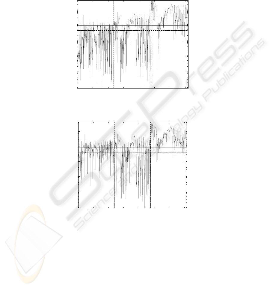
process is illustrated by the variation in the Q statistic shown in Figure 6.
1000 2000 3000 4000 5000 6000 7000 8000 9000
10
-5
10
-4
10
-3
10
-2
data points
Q (log)
RM
ET
Fig. 6. Q statistic variation on fault-free MI cycle data collected under two atmospheric
temperature conditions for model validation.
36

Here the upper limit represents the 99% confidence level, whereas the lower one is
for a 95% threshold, both of which were derived from the Q statistic of the AANN
training data. The resulting numbers of violations shown for data recorded under both
the RM and ET conditions are statistically acceptable, confirming the modelling
validity of the trained AANN.
4.2 Generalisation
When a model is used in practice, the new operational inputs often take a form
previously unseen by the model during its training. This is particularly the case with
automotive IC engines, which impose a stringent requirement for generalisation if the
results are to be of practical significance. This aspect of the NLPCA model was
therefore challenged by comparing the measured and predicted values of both mass
air flow and manifold air pressure produced by the NEDC with the engine operating
under fault-free conditions. The excellent generalisation capability of the trained
AANN is supported by
Fig. 7, which shows the low numbers of violations of the
confidence limits by the Q statistic under both temperature conditions. This reveals
that there is little difference between the measured engine data and the corresponding
predictions. This is an important finding as the NEDC engine inputs of speed and
pedal position vary at rates ranging from steady-state up to the highly transient
conditions found during 1st gear accelerations and motored deceleration phases.
Moreover, the atmospheric conditions when these data sets were collected also
differed from those of the training data.
0.5 1 1.5 2
x 10
4
10
-5
10
-4
10
-3
10
-2
data points
Q (log)
RM
ET
Fig. 7. Q statistic variation on fault-free NEDC and two temperature conditions for model
generalisation.
4.3 Fault Detection on MI Data
This section assesses the AANN model’s ability to detect a fault produced by running
the MI cycle in the presence of a 2mm, 4mm, and 6mm air leak on the inlet manifold.
Fig. 8 and Fig. 9 show the variation in the corresponding Q statistics for data recorded
under RM and ET conditions respectively. It can be seen that in either case the
37
number of violations of the confidence limits naturally grows as the magnitude of the
fault increases. Since the 2mm air leak does not have a significant impact on the
engine performance, its Q statistic does not produce as many obvious violations to the
99% confidence limits as for the larger two air leaks. Even so, this minor fault can
still be detected by referencing to the 95% confidence limit.
2000 4000 6000 8000 10000 12000 14000
10
-6
10
-5
10
-4
10
-3
10
-2
10
-1
data points
Q (log)
2mm 4mm 6mm
Fig. 8. Monitoring 2mm/4mm/6mm air leak faults for the MI cycle at the RM temperature
condition.
2000 4000 6000 8000 10000 12000 14000
10
-6
10
-5
10
-4
10
-3
10
-2
10
-1
data points
Q (log)
2mm
4mm
6mm
Fig. 9. Monitoring 2mm/4mm/6mm air leak faults for the MI cycle at the ET temperature
condition.
It should be noted that there are certain regions in the faulty data set where the
impact of the air leak fault may not be apparent in the monitoring statistic. This is
expected, as this fault would not affect the engine when it is operating at high throttle
openings. Under such circumstances, the manifold pressure is close to, or equal to, the
atmospheric pressure. Consequently, the pressure difference across the leakage orifice
is small and the flow rate of air through it is therefore negligible.
38
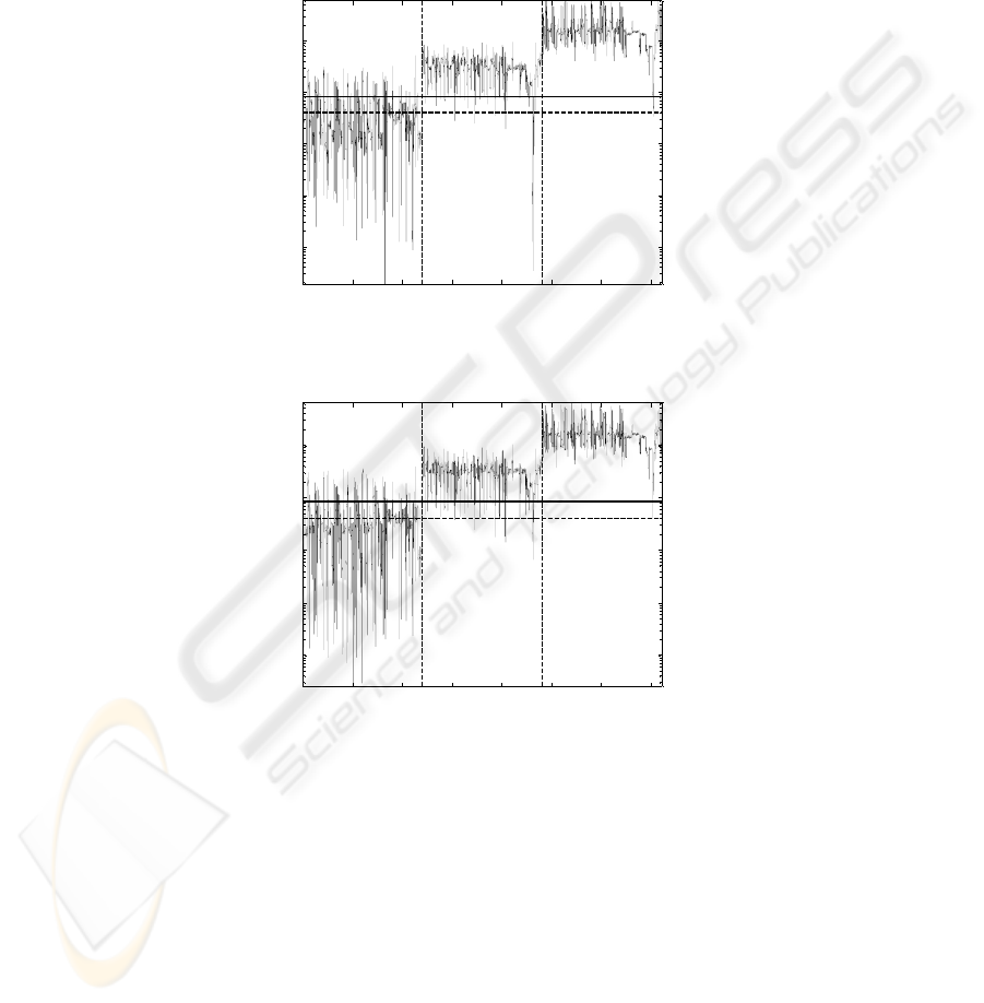
4.4 Fault Detection on NEDC
The variations in Q statistic for the AANN model shown in
Fig. 10 and Fig. 11 cover
the three fault conditions for the NEDC under both RM and ET temperature
conditions respectively. Pleasingly, these results confirm successful detection of all
three air leak faults, despite the model having being trained using the substantially
different MI identification cycle.
0.5 1 1.5 2 2.5 3 3.5
x 10
4
10
-5
10
-4
10
-3
10
-2
10
-1
data points
Q (log)
2mm 4mm 6mm
Fig. 10. Monitoring 2mm/4mm/6mm air leak faults for the NEDC cycle at the RM temperature
condition.
0.5 1 1.5 2 2.5 3 3.5
x 10
4
10
-5
10
-4
10
-3
10
-2
10
-1
data points
Q (log)
2mm
4mm 6mm
Fig. 11. Monitoring 2mm/4mm/6mm air leak faults for the NEDC cycle at the ET temperature
condition.
5 Conclusions
This paper showed the capability of an AANN in both modelling and air-leak fault
detection for an automotive gasoline IC engine. The modelling data was derived for
two different transient drive cycles under different atmospheric temperature
conditions. The model trained using MI cycle data sets that were recorded under all
39

available atmospheric temperature conditions produced the best generalisation to
measurements from the unseen NEDC cycle. There was an absence of unwanted false
alarms under fault-free conditions, and successful detection of air leaks of varying
magnitude in the inlet manifold.
Acknowledgements
The authors are grateful to the U.K. Engineering and Physical Science Research
Council (Grant No. EP/C005457) for their financial support.
References
1. Antory, D., U. Kruger, G.W. Irwin and G. McCullough 2005. Fault diagnosis in internal
combustion engines using nonlinear multivariate statistics. Proc Institution of Mechanical
Engineers, Part I: Journal of Systems and Control Engineering, 219(4), 243-258.
2. Crossman, J.A., H. Guo, Y.K. Murphey and J. Cardillo 2003. Automotive signal fault
diagnostics – part I: signal fault analysis, signal segmentation, feature extraction and quasi-
optimal feature selection. IEEE Transactions on Vehicular Technology 52(4), 1063-1075.
3. Grimaldi, C.N. and F. Mariani 2001. OBD Engine Fault Detection Using a Neural
Approach. SAE Paper No. 2001-01-0559.
4. Jackson, J.E. 1991. A Users Guide to Principal Components. Wiley Series in Probability
and Mathematical Statistics. John Wiley, New York.
5. Kimmich, F., A. Schwarte and R. Isermann 2005. Fault detection for modern diesel engines
using signal- and process model-based methods. Control Engineering Practice 13, 189-203.
6. Kramer, M.A. 1992. Autoassociative neural networks. Computers and Chemical
Engineering 16(4), 313-328.
7. Nyberg, M. 1999. Model Based Diagnosis of Both Sensor Faults and Leakage in the Air-
Intake System of an SI Engine. SAE Paper No. 1999-01-0860.
8. Sher, E. 1984. Effect of atmospheric conditions on the performance of an air-borne two-
stroke spark-ignition engine. Proc Institution of Mechanical Engineers, Part D: Transport
Engineering. 198(15), 239-251.
9. Stobart, R. 2003. Control oriented models for exhaust gas aftertreatment; A Review and
Prospects, SAE Paper No. 2003-01-1004.
10. Wang, X., U. Kruger, G.W. Irwin, G. McCullough and N. McDowell 2008a. Nonlinear
PCA with the local approach for diesel engine fault detection and diagnosis, IEEE Trans.
Control Systems Technology 16 (1), 122-129
11. Wang, X., G.W. Irwin, G. McCullough, N. McDowell and U. Kruger 2008b. Application of
nonlinear dynamic PCA to automotive engine modelling and fault monitoring, Control
Engineering
40
