
A
BAYESIAN APPROACH TO 3D OBJECT RECOGNITION USING
LINEAR COMBINATION OF 2D VIEWS
Vasileios Zografos and Bernard F. Buxton
Department of Computer Science, University College London, Malet Place, London, WC1E 6BT, UK
Keywords:
Object recognition, linear combination of views, Bayes, Markov-Chain Monte-Carlo.
Abstract:
We introduce Bayes priors into a recent pixel-based, linear combination of views object recognition technique.
Novel views of an object are synthesized and matched to the target scene image using numerical optimisation.
Experiments on a real-image, public database with the use of two different optimisation methods indicate
that the priors effectively regularize the error surface and lead to good performance in both cases. Further
exploration of the parameter space has been carried out using Markov Chain Monte Carlo sampling.
1 INTRODUCTION
In this work, we examine computational aspects of
a pixel-based linear combination of views approach
to the recognition of objects that vary due to changes
in the viewpoint from which they can be seen. This
method works directly with a search over pixel val-
ues and avoids the need for low-level feature extrac-
tion and solution of the correspondence problem. In
this paper we illustrate how, by using a Bayesian ap-
proach, we can restrict our search to regions where
valid and meaningful solutions are likely to exist.
The method works by recovering a set of linear
coefficients that will combine a small number of 2-
D views of an object and synthesise a novel image
which is as similar as possible to a target image of
the object. Bayes priors are constructed and shown to
regularize optimisation of the synthesized image. For
one selected object recognition example, Monte Carlo
Markov Chain (MCMC) sampling is used to explore
the form of the posterior distribution.
2 PROPOSED METHOD
By using the linear combination of views (LCV) the-
ory (Shashua, 1995; Ullman and Basri, 1991) we can
deal with the variations in an object’s appearance due
to viewpoint changes. Thus, given two different views
I
0
(x
0
,y
0
) and I
00
(x
00
,y
00
) of an object (Fig. 1(a), (b)), we
can represent any corresponding point (x, y) in a novel
target image I
T
as:
x = a
0
+ a
1
x
0
+ a
2
y
0
+ a
3
x
00
+ a
4
y
00
y = b
0
+ b
1
x
0
+ b
2
y
0
+ b
3
x
00
+ b
4
y
00
. (1)
These equations are overcomplete (Ullman and Basri,
1991) and other choices may be made (Koufakis and
Buxton, 1998). The novel view may then be synthe-
sised by warping and blending the images I
0
and I
00
as
follows:
I
T
(x, y) = w
0
I
0
(x
0
,y
0
) + w
00
I
00
(x
00
,y
00
) + ε(x, y). (2)
Only 5 or more corresponding landmark points are
necessary in the two views (Fig. 1(a), (b)), and the
weights w
0
and w
00
are calculated as described in (Ko-
ufakis and Buxton, 1998).
We extend (1) and (2) by incorporating prior infor-
mation on the coefficients (a
i
,b
j
), based on previous
training with synthetic data, and building a Bayesian
model. On the assumption that ε(x, y) in (2) is i.i.d.
random noise drawn from a Gaussian distribution and
similarly using Gaussian priors for the LCV coeffi-
cients (here considered statistically independent) with
means and standard deviations estimated from train-
ing data, we get the log posterior as, devoid of any
uninteresting constants:
295
Zografos V. and F. Buxton B. (2008).
A BAYESIAN APPROACH TO 3D OBJECT RECOGNITION USING LINEAR COMBINATION OF 2D VIEWS.
In Proceedings of the Third International Conference on Computer Vision Theory and Applications, pages 295-298
DOI: 10.5220/0001081902950298
Copyright
c
SciTePress

(a) (b)
(c) (d)
Figure 1: Example of real data from the COIL-20 database.
The two basis view images I
0
(a) and I
00
(b) with landmark
points selected at prominent features. I
T
(c) is the target im-
age. The synthesised image (d) is at the correct pose identi-
fied by our algorithm. .
−log[P(~a
i
,
~
b
j
|I
T
,I
0
,I
00
)] ∝
∑
x,y
[I
T
(x,y)−I
S
(x,y)]
2
σ
2
ε
+
∑
4
i=0
(~a
i
−µ
a
i
)
2
σ
2
a
i
+
∑
4
j=0
(
~
b
j
−µ
b
j
)
2
σ
2
b
j
.
(3)
This defines the probability of observing the target
image I
T
given the vectors of coefficients (~a
i
,
~
b
j
) and
the basis views I
0
and I
00
. We usually require a single
synthesised image to be presented as the most prob-
able result. A typical choice is the one which max-
imises the posterior probability (MAP) or minimises
the negative log-posterior (3) with respect to the pa-
rameters a
i
and b
j
. The latter can be minimised using
standard optimisation techniques.
Priors were constructed by examination of the
variation of the LCV coefficients using a synthetic 3D
model. It was found that a
0
follows a quadratic curve,
coefficients a
1
and a
3
are linear whilst the remaining
coefficients are almost constant. Appropriate Gaus-
sian priors were defined whose effect can be seen in
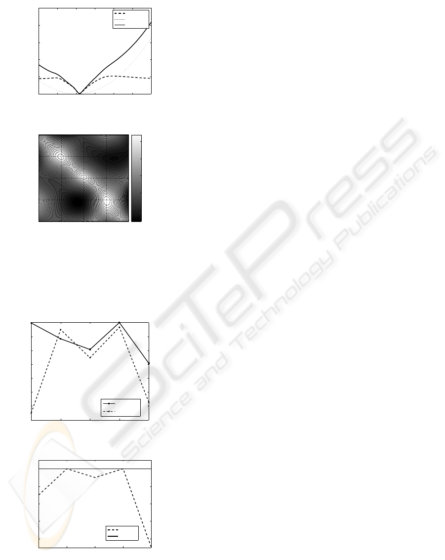
Fig. 2(a). Here we show negative log probability of
the likelihood, prior and posterior for the coefficient
a
2
. The plot was generated by isolating and varying
this coefficient while having conditioned the remain-
ing coefficients to the optimal prior values identified
previously during training. We note the effect of the
prior on the likelihood, especially near the tails of the
p.d.f. where we have large error residuals. The prior
widens the likelihood’s basin of attraction resulting
in much easier minimisation, even if we initialise our
optimisation algorithm far away from the optimal so-
lution.
On the other hand, near the global optimum we
wish the prior to have as little impact as possible in
order for the detailed information as to the value of
a
2
to come from the likelihood alone. This allows
for small deviations from the values for the coeffi-
cients encoded in the prior means, since every synthe-
sis and recognition problem differs slightly due to ob-
ject type, location, orientation and perspective camera
effects.
Using the LCV for object recognition is straight-
forward. The first component of our system is the
two stored basis views I
0
and I
00
which define the li-
brary of known modelled objects. These are rectangu-
lar bitmap images that contain grey-scale (or colour)
pixel information of the object without any additional
background data. It is important not to choose a very
wide angle between the basis views to avoid I
0
and I
00
belonging to different aspects of the object with land-
mark points being occluded.
Having selected the two basis views, we pick a
number of corresponding landmark points, in par-
ticular lying on edges and other prominent fea-
tures. We then use constrained Delaunay triangula-
tion (Shewchuk, 2002) and the correspondence to pro-
duce similar triangulations on both the images. The
above processes may be carried out during an off-line,
model-building stage and are not examined here.
The set of LCV coefficients is then determined by
minimising the negative log posterior (3) and the ob-
ject of interest in the target image I
T
recognised by
selecting the best of the models, as represented by
the basis views, that explain I
T
sufficiently well. Es-
sentially, we are proposing a flexible template match-
ing system in which the template is allowed to de-
form in the LCV space, restricted by the Bayesian
priors to regions where there is a high probability of
meaningful solutions, until it matches the target im-
age. To do this we need to search a high-dimensional
parameter space using an efficient optimisation algo-
rithm. We have tested Differential Evolution (Storn
and Price, 1997) and a reformulation of the simplex
algorithm (Zografos and Buxton, 2007; Nelder and
Mead, 1965).
3 EXPERIMENTS
We have performed a number of experiments on real
images using the publicly available COIL-20 database
(Nene et al., 1996). This database contains exam-
ples of 20 objects imaged under varying pose (hori-
zontal rotation around the view-sphere at 5
o
intervals)
against a constant background with the camera posi-
tion and lighting conditions kept constant. We con-
structed LCV models from 5 objects, using as basis
views the images at ±20
o
from a frontal view, while
VISAPP 2008 - International Conference on Computer Vision Theory and Applications
296
−2 −1 0 1 2 3 4
0
2
4
6
8
10
x 10
4
a
2
−log probability
Likelihood
Prior
Posterior
(a)
Image
Model
1 3 5 7 9
1
3
5
7
9
0.5
0.6
0.7
0.8
0.9
(b)
Figure 2: (a) The negative log posterior resulting from the
combination of the prior and likelihood. (b) Model × im-
age heatmap array with high cross-correlation in the main
diagonal.
1 3 5 7 9
0.82
0.84
0.86
0.88
0.9
0.92
0.94
0.96
Model
Cross correlation
Responses averaged over test runs
DE
Simplex
(a)
1 3 5 7 9
20
40
60
80
100
Model
Recognition percentage %
Recognition % averaged over test runs
Simplex
DE
(b)
Figure 3: (a) Comparison of the average response between
the DE and simplex algorithm and (b) their average recog-
nition rates on the same dataset.
ensuring that the manually chosen landmarks were
visible in both I
0
and I
00
(Fig. 1). Comparisons were
carried out against target images from the same set of
modelled objects taken in the frontal pose at 0
o
.
In total, we carried out 500 experiments (250 with
each optimisation method × 10 tests for each model-
target image combination) and constructed two 5 × 5
arrays of model×image results. Each array contains
information about the matching scores represented by
the cross-correlation coefficient. The highest scores
were along the main diagonal where each model of
an object is correctly matched to a target image of the
same object.
For the simplex method, we set the maximum
number of function evaluations (NFEs) to 1000 and a
fixed initialisation of: a
o
,a
1
,a
3
,b
0
,b
1
=1, a
2
,a
4
,b
3
=0.5,
b
2
=0.9, b
4
=1.4, deliberately chosen far away from the
expected prior solution in order not to influence the
optimisation algorithm with a good initialisation. In
the case of DE, we chose a much higher NFEs=20000
(100 populations × 200 generations) and specified
the boundaries of the LCV space as: -5≤ a
0
,b
0
≤5,
-1≤ a
1
,a
2
,a
3
,a
4
≤1, -1≤ b
1
,b
2
,b
3
,b
4
≤1.
The results of the above experiments, averaged
over 10 test runs, are summarised in the heatmap plot
Fig. 2(b). As expected, we can see a well defined
diagonal of high cross-correlation where the correct
model is matched to the target image. This obser-
vation, combined with the absence of any significant
outlying good matches when model6=image, leads us
to the conclusion that, on average, both methods per-
form well in terms of recognition results. The ques-
tion is how close these methods can get to the global
optimum, and in how great a NFEs.
We have also included the plots in Fig. 3(a) and
(b) which compare the average cross-correlation re-
sponses and the recognition rates for both methods re-
spectively. A recognition is deemed a failure if the re-
covered cross-correlation value is below the 95
th
per-
centile of the ground truth solution in each case. This
threshold is empirical and some test runs with much
lower scores produce visually acceptable matching re-
sults.
Both methods have a consistently good perfor-
mance with the DE converging to solutions of higher
cross-correlation in most cases while producing re-
sults over 95% of the ground truth in every case. The
simplex failed to converge to the correct solution in a
few cases, particularly in some of the tests for models
1 and 9, while producing acceptable recognition re-
sults in the majority of test runs. This of course may
be explained in part by the smaller NFEs that were
allowed for this algorithm although preliminary ex-
periments had indicated the NFE value chosen should
A BAYESIAN APPROACH TO 3D OBJECT RECOGNITION USING LINEAR COMBINATION OF 2D VIEWS
297

generally have sufficed.
From these experiments we have also observed
that there is little diversity in the 10 coefficients in
the recovered solutions along the main diagonal in-
dicating a stability in the coefficients across different
objects that is consistent with the prior training data.
Also, we have detected a difference in the optimisa-
tion behaviour of the two algorithms, DE and sim-
plex, and how much earlier the latter can reach the
global minimum. DE is much slower, but it has the
advantage that it can avoid locally optimum solutions,
which the simplex sometimes cannot.
Finally, in order to obtain a more specific and
complete idea of the characteristics of the posterior
surface, we have used a Markov-Chain Monte Carlo
(MCMC) (Gelman et al., 1995) approach in order to
generate a sample of the distribution and further anal-
yse it. We chose a single experiment (matching to a
frontal view of object 1 at 0
0
) and generated a set of
10000 samples of the posterior (3) from areas of high
probability using a single Markov Chain. We then ran
a k-means clustering algorithm (Bishop, 1995) which
recovered 3 main clusters in close proximity and all
near the global optimum. This indicates that, for this
example, the distribution is approximately unimodal
though perhaps with some subsidiary, nearby peaks
caused by noise effects. The main point is that there
is no significant local optimum elsewhere nearby in
the distribution.
A final examination of the kurtosis and skew-
ness of the sample has shown that the distributions
of the samples of all coefficients, except b
1
, are quite
strongly skewed, reflecting strong influence of the
likelihood near the optimum posterior, a property that
is highly desirable. This is due to the shape of the
likelihood function since the priors are symmetric.
The values for the kurtosis are small for some coeffi-
cients whose posteriors are therefore almost Gaussian
near the optimum, whilst other coefficients strongly
affected by the priors are leptokurtic.
4 CONCLUSIONS
Our approach to view-based object recognition in-
volves synthesising intensity images using a linear
combination of views and comparing the sythesised
images to the target, scene image. We incorporate
prior probabilistic information on the LCV parame-
ters by means of a Bayesian model. Matching and
recognition experiments carried out on data from the
COIL-20 public database have shown that our method
works well for pose variations where the target view
lies between the basis views. The experiments further
show the beneficial effects of the prior distributions in
“regularising” the optimisation. In particular, priors
could be chosen that produced a good basin of attrac-
tion surrounding the desired optimum without unduly
biasing the solution.
Nevertheless, additional work is required. In order
to avoid the overcompleteness of the LCV equations,
we would like to reformulate the LCV equations (1)
by using the affine tri-focal tensor and introducing the
appropriate constraints in the LCV mapping process.
In addition, in this paper we have only addressed ex-
trinsic viewpoint variations, but it should also be pos-
sible to include intrinsic, shape variations using the
approach described by (Dias and Buxton, 2005).
REFERENCES
Bishop, C. M. (1995). Neural Networks for Pattern Recog-
nition. Oxford University Press.
Dias, M. B. and Buxton, B. F. (2005). Implicit, view invari-
ant, linear flexible shape modelling. Pattern Recogni-
tion Letters, 26(4):433–447.
Gelman, A., Carlin, J. B., Stern, H. S., and Rubin, D. B.
(1995). Bayesian Data Analysis. Chapman and Hall,
London, 2nd edition.
Koufakis, I. and Buxton, B. F. (1998). Very low bit-rate
face video compression using linear combination of
2dfaceviews and principal components analysis. Im-
age and Vision Computing, 17:1031–1051.
Nelder, J. A. and Mead, R. (1965). A simplex method
for function minimization. Computer Journal, 7:308–
313.
Nene, S. A., Nayar, S. K., and Murase, H. (1996). Columbia
Object Image Library (COIL-20). Technical Re-
port CUCS-006-96, Department of computer science,
Columbia University, New York, N.Y. 10027.
Shashua, A. (1995). Algebraic functions for recognition.
IEEE Transactions on Pattern Analysis and Machine
Intelligence, 17(8):779–789.
Shewchuk, J. R. (2002). Delaunay refinement algorithms
for triangular mesh generation. Computational Ge-
ometry: Theory and Applications, 22:21–74.
Storn, R. and Price, K. V. (1997). Differential evolution - a
simple and efficient heuristic for global optimization
overcontinuous spaces. Journal of Global Optimiza-
tion, 11(4):341–359.
Ullman, S. and Basri, R. (1991). Recognition by linear com-
binations of models. IEEE Transactions on Pattern
Analysis and Machine Intelligence, 13(10):992–1006.
Zografos, V. and Buxton, B. F. (2007). Pose-invariant
3d object recognition using linear combination of 2d
views and evolutionary optimisation. ICCTA, pages
645–649.
VISAPP 2008 - International Conference on Computer Vision Theory and Applications
298
